🚀 What is the Law of Large Numbers?

In probability theory, the Law of Large Numbers is a mathematical law that states that the average of the results obtained from a large number of independent random samples converges to the true value, if it exists.

In general, this theorem says that if you repeat the same random experiment many times under the same conditions, the sample average will get closer and closer to the true mean (also called the population mean).

Formally, for random variables \(X_1, X_2,\ldots\) with a finite mean \(\mu\), the sample mean approaches \(\mu\) as \(n\) grows.

It may be stimated using the equation: \[ \overline{X}_n \;=\; \frac{1}{n}\sum_{i=1}^{n} X_i, \]

🪙 Example: Coin Flips (Heads = 1, Tails = 0)

Let’s simulate the Law of Large Numbers using a classic example — flipping a fair coin.

For a fair coin, the chance is 0.05 \(\Rightarrow\) \(\mathbb{E}[X]=0.5\).

Below I simulated many flips and track the running average to show it drifting toward 0.5.

library(ggplot2)

# seed

set.seed(123)

# number of flips
n <- 2000 

# trials
x <- rbinom(n, size = 1, prob = 0.5)  # Heads=1, Tails=0

# cummulative means
running_mean <- cumsum(x) / seq_along(x)

df <- data.frame(
  trial = 1:n,
  running_mean = round(running_mean, 2))

👀 Take a look at the first 10 and the last 10 experiments.

df |> 
  dplyr::select(trial,running_mean) |>
  dplyr::slice_head(n = 10)

##    trial running_mean
## 1      1         0.00
## 2      2         0.50
## 3      3         0.33
## 4      4         0.50
## 5      5         0.60
## 6      6         0.50
## 7      7         0.57
## 8      8         0.62
## 9      9         0.67
## 10    10         0.60

df |> 
  dplyr::select(trial,running_mean) |>
  dplyr::slice_tail(n = 10)

##    trial running_mean
## 1   1991          0.5
## 2   1992          0.5
## 3   1993          0.5
## 4   1994          0.5
## 5   1995          0.5
## 6   1996          0.5
## 7   1997          0.5
## 8   1998          0.5
## 9   1999          0.5
## 10  2000          0.5

🎨 Let’s plot the simulation

df |>
  ggplot(aes(trial, running_mean)) +
  geom_line(linewidth = 0.8) +
  geom_hline(yintercept = 0.5, 
             linetype = "dashed",
             color = "red", 
             linewidth = 0.6) +
  scale_y_continuous(limits = c(0, 0.8)) +
  labs(
    title = "Running Average of Coin Flips Converges to 0.5 🎯",
    subtitle = "Law of Large Numbers in action",
    x = "Number of flips",
    y = "Running average"
  ) +
  ggthemes::theme_economist()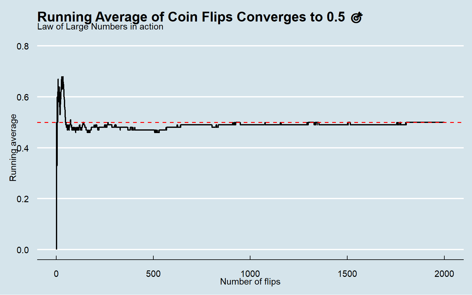

👀 What can we see and Practical Applications⚠️

Again, as expected, in the early experiments, the sample mean fluctuates considerably, but as the number of experiments grows, it steadily converges to the true value (0.5).

It justifies using sample means for estimation in distinct areas, for instance:

• 🧪 Clinical trials (research): Averaging patient outcomes across many participants makes the treatment effect stabilize around its true value, supporting reliable estimates of efficacy and safety.

• 🧫 A/B testing: With more users, average conversion rates settle near the true rates, letting teams decide which variant truly performs better.

• 🗳️ Polling & surveys: Larger, well-sampled polls yield averages (approval, intention to vote, prevalence) that home in on population values.

• 🏭 Quality control: Averaging defect counts or measurements over many items reveals the true process mean, guiding process adjustments and Six Sigma targets.

• 🧮 Monte Carlo simulation: Sample means of simulated outcomes converge to expected values, underpinning pricing (e.g., options), reliability estimation, and uncertainty quantification.

• 🧾 Econometrics & big data: Estimators built from sample averages (moments, means, residuals) become stable with large datasets, improving inference and model selection.

• 🧑‍⚕️ Epidemiology & public health: Averaging incidence or biomarker readings across large cohorts yields stable estimates of prevalence, risk factors, and baseline rates.

References

• Book - Dekking, et al A Modern Introduction to Probability and Statistics;

• Wikipedia - Law of large numbers