Using Random Forest to Predict Heart Disease
By Saulo Gil
February 6, 2024
Introduction
Heart disease, also known as cardiovascular disease (CVDs), encompasses a range of conditions that affect the heart and blood vessels. It is the leading cause of death globally. It consists to a group of disorders that affect the heart and blood vessels such as coronary artery disease, stroke, peripheral artery disease, hypertension and, heart failure. It is noteworthy that CVDs are the number 1 cause of death globally, taking an estimated 17.9 million lives each year, which accounts for 31% of all deaths worldwide.
Heart disease are the number 1 cause of death globally, taking an estimated 17.9 million lives each year, which accounts for 31% of all deaths worldwide. Indeed, CVDs can significantly impact mortality rates, especially if left untreated or poorly managed. Early diagnosis and management of risk factors can help prevent heart disease and improve outcomes for those living with the condition.
Random Forest is a popular machine learning algorithm used for both classification and regression tasks. It consists of multiple random decision trees. Briefly, two types of randomnesses are built into the trees. First, each tree is built on a random sample from the original data. Second, at each tree node, a subset of features is randomly selected to generate the best split. Thus, it is reasonable to assume that this machine learning algorithm may be useful for the early detection and treatment of heart disease and, finally, for avoiding complications and improving outcomes.
Herein, we utilized the Random Forest to predict cardiovascular disease.
Packages
# Pacotes
library(tidyverse)
library(tidymodels)
library(GGally)
library(DataExplorer)
library(doParallel)
Reading dataset
This data set dates from 1988 and consists of four databases: Cleveland, Hungary, Switzerland, and Long Beach V. It contains 76 attributes, including the predicted attribute, but all published experiments refer to using a subset of 14 of them. The “target” field refers to the presence of heart disease in the patient. It is integer valued 0 = no disease and 1 = disease.
The features are following:
age;
sex;
chest pain type (4 values);
resting blood pressure;
serum cholestoral in mg/dl;
fasting blood sugar > 120 mg/dl;
resting electrocardiographic results (values 0,1,2);
maximum heart rate achieved;
exercise induced angina;
oldpeak = ST depression induced by exercise relative to rest;
the slope of the peak exercise ST segment;
number of major vessels (0-3) colored by flourosopy;
thal: 0 = normal; 1 = fixed defect; 2 = reversable defect.
Let’s load the dataset!
# Lendo a base
df <- read.csv('heart.csv') |>
  janitor::clean_names() |> #lowercase columns
  mutate(
    heart_disease = as.factor(heart_disease)
  )
Pre-processing
Pre-processing of data is a crucial step for preparing and cleaning the dataset before feeding it into a machine learning model. It plays a significant role in improving the performance, accuracy, and reliability of the model. Therefore, let’s deep into the dataset!!!
Looking the outcome (heart disease)
df |>
  ggplot(mapping = aes(x = heart_disease, fill = sex)) +
  geom_bar() +
  theme_bw()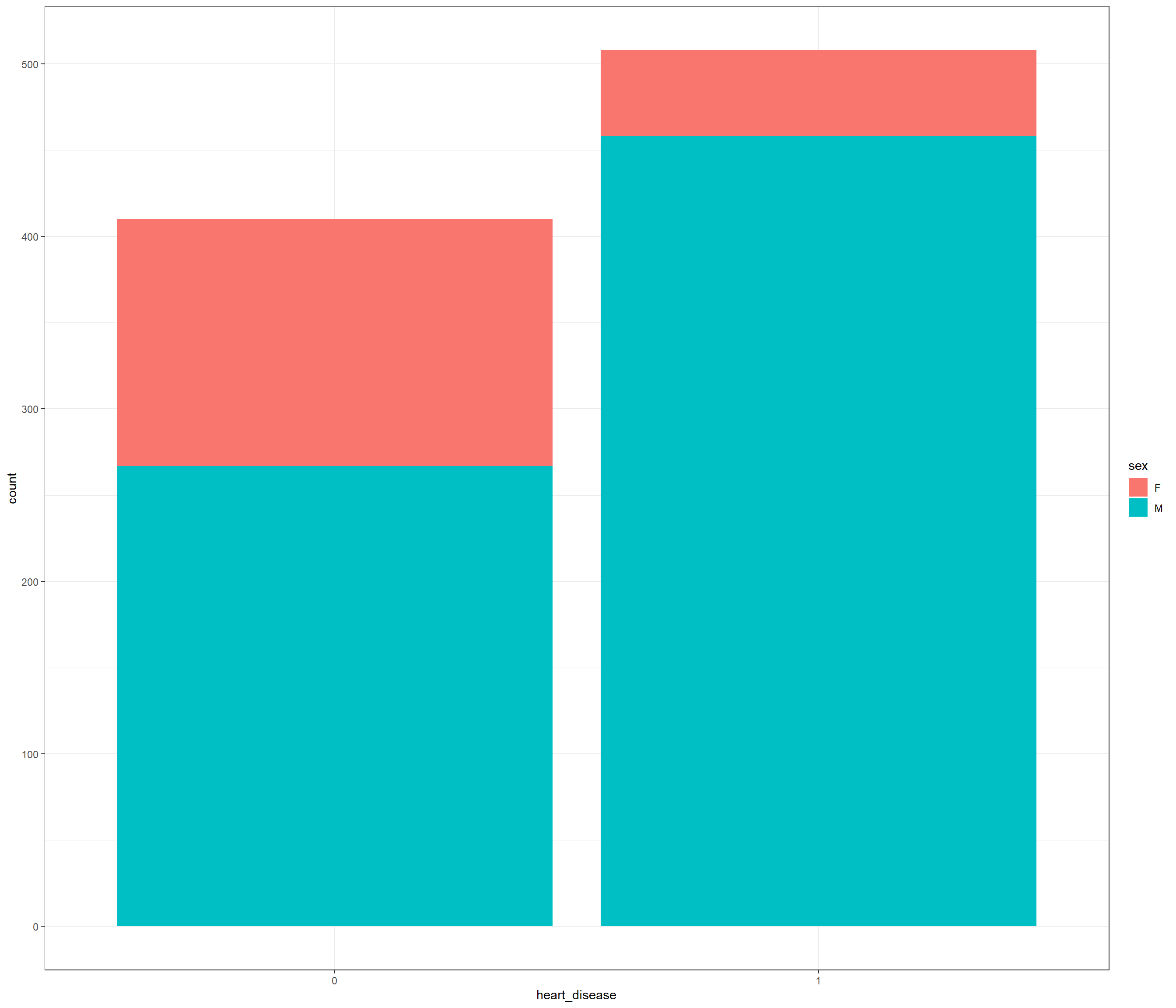
df |>
  count(heart_disease)
## heart_disease n
## 1 0 410
## 2 1 508The number of classes of the outcome seems balanced!
Data engineering
df_adjust <-
  df |>
  mutate(
    # sex for dummies
    sex = case_when(sex == "M" ~ "0",
                    sex == "F" ~ "1"),
    # creating dummies for chest_pain_type
    chest_pain_type_ATA = case_when(chest_pain_type == "ATA" ~ 1,
                                    chest_pain_type != "ATA" ~ 0),
    chest_pain_type_NAP = case_when(chest_pain_type == "NAP" ~ 1,
                                    chest_pain_type != "NAP" ~ 0),
    chest_pain_type_ASY = case_when(chest_pain_type == "ASY" ~ 1,
                                    chest_pain_type != "ASY" ~ 0),
    chest_pain_type_TA = case_when(chest_pain_type == "TA" ~ 1,
                                    chest_pain_type != "TA" ~ 0),
    # creating dummies for resting_ecg
    resting_ecg_normal = case_when(resting_ecg == "Normal" ~ 1,
                                   resting_ecg != "Normal" ~ 0),
    resting_ecg_st = case_when(resting_ecg == "ST" ~ 1,
                               resting_ecg != "ST" ~ 0),
    resting_ecg_lvh = case_when(resting_ecg == "LVH" ~ 1,
                                 resting_ecg != "LVH" ~ 0),
    # creating dummies for exercise_angina
    exercise_angina = case_when(exercise_angina == "Y" ~ 1,
                                exercise_angina == "N" ~ 0),
    # creating dummies for st_slope
    st_slope_up = case_when(st_slope == "Up" ~ 1,
                            st_slope != "Up" ~ 0),
    st_slope_flat = case_when(st_slope == "Flat" ~ 1,
                            st_slope != "Flat" ~ 0),
    st_slope_down = case_when(st_slope == "Down" ~ 1,
                            st_slope != "Down" ~ 0)
    ) |>
  # selecting features
  select(age,
         sex,
         resting_bp,
         cholesterol,
         fasting_bs,
         max_hr,
         oldpeak,
         chest_pain_type_ATA,
         chest_pain_type_NAP,
         chest_pain_type_ASY,
         chest_pain_type_TA,
         resting_ecg_normal,
         resting_ecg_st,
         resting_ecg_lvh,
         exercise_angina,
         st_slope_up,
         st_slope_flat,
         st_slope_down,
         heart_disease
         ) |>
  #adjusting type of data
  mutate(sex = as.character(sex),
         fasting_bs = as.character(fasting_bs),
         chest_pain_type_ATA = as.character(chest_pain_type_ATA),
         chest_pain_type_NAP = as.character(chest_pain_type_NAP),
         chest_pain_type_ASY = as.character(chest_pain_type_ASY),
         chest_pain_type_TA = as.character(chest_pain_type_TA),
         resting_ecg_normal = as.character(resting_ecg_normal),
         resting_ecg_st = as.character(resting_ecg_st),
         resting_ecg_lvh = as.character(resting_ecg_lvh),
         exercise_angina = as.character(exercise_angina),
         st_slope_up = as.character(st_slope_up),
         st_slope_flat = as.character(st_slope_flat),
         st_slope_down = as.character(st_slope_down)
         )

glimpse(df_adjust)
## Rows: 918
## Columns: 19
## $ age <int> 40, 49, 37, 48, 54, 39, 45, 54, 37, 48, 37, 58, 39…
## $ sex <chr> "0", "1", "0", "1", "0", "0", "1", "0", "0", "1", …
## $ resting_bp <int> 140, 160, 130, 138, 150, 120, 130, 110, 140, 120, …
## $ cholesterol <int> 289, 180, 283, 214, 195, 339, 237, 208, 207, 284, …
## $ fasting_bs <chr> "0", "0", "0", "0", "0", "0", "0", "0", "0", "0", …
## $ max_hr <int> 172, 156, 98, 108, 122, 170, 170, 142, 130, 120, 1…
## $ oldpeak <dbl> 0.0, 1.0, 0.0, 1.5, 0.0, 0.0, 0.0, 0.0, 1.5, 0.0, …
## $ chest_pain_type_ATA <chr> "1", "0", "1", "0", "0", "0", "1", "1", "0", "1", …
## $ chest_pain_type_NAP <chr> "0", "1", "0", "0", "1", "1", "0", "0", "0", "0", …
## $ chest_pain_type_ASY <chr> "0", "0", "0", "1", "0", "0", "0", "0", "1", "0", …
## $ chest_pain_type_TA <chr> "0", "0", "0", "0", "0", "0", "0", "0", "0", "0", …
## $ resting_ecg_normal <chr> "1", "1", "0", "1", "1", "1", "1", "1", "1", "1", …
## $ resting_ecg_st <chr> "0", "0", "1", "0", "0", "0", "0", "0", "0", "0", …
## $ resting_ecg_lvh <chr> "0", "0", "0", "0", "0", "0", "0", "0", "0", "0", …
## $ exercise_angina <chr> "0", "0", "0", "1", "0", "0", "0", "0", "1", "0", …
## $ st_slope_up <chr> "1", "0", "1", "0", "1", "1", "1", "1", "0", "1", …
## $ st_slope_flat <chr> "0", "1", "0", "1", "0", "0", "0", "0", "1", "0", …
## $ st_slope_down <chr> "0", "0", "0", "0", "0", "0", "0", "0", "0", "0", …
## $ heart_disease <fct> 0, 1, 0, 1, 0, 0, 0, 0, 1, 0, 0, 1, 0, 1, 0, 0, 1,…Done!!! Lest’s explore the dataset.
Spliting dataset - Train/Test
Since our dataset is size-limited (n-918), I opted to separate 70% of the sample size for training.
set.seed(32)

heart_initial_split <- initial_split(df,
                                     prop = 0.7,
                                     strata = "heart_disease")
heart_initial_split
## <Training/Testing/Total>
## <642/276/918># train and test datasets
heart_train <- training(heart_initial_split)
heart_test <- testing(heart_initial_split)Exploratory analysis
Overview
skimr::skim(heart_train)| Name | heart_train |
| Number of rows | 642 |
| Number of columns | 12 |
| _______________________ | |
| Column type frequency: | |
| character | 5 |
| factor | 1 |
| numeric | 6 |
| ________________________ | |
| Group variables | None |
Variable type: character
| skim_variable | n_missing | complete_rate | min | max | empty | n_unique | whitespace |
|---|---|---|---|---|---|---|---|
| sex | 0 | 1 | 1 | 1 | 0 | 2 | 0 |
| chest_pain_type | 0 | 1 | 2 | 3 | 0 | 4 | 0 |
| resting_ecg | 0 | 1 | 2 | 6 | 0 | 3 | 0 |
| exercise_angina | 0 | 1 | 1 | 1 | 0 | 2 | 0 |
| st_slope | 0 | 1 | 2 | 4 | 0 | 3 | 0 |
Variable type: factor
| skim_variable | n_missing | complete_rate | ordered | n_unique | top_counts |
|---|---|---|---|---|---|
| heart_disease | 0 | 1 | FALSE | 2 | 1: 355, 0: 287 |
Variable type: numeric
| skim_variable | n_missing | complete_rate | mean | sd | p0 | p25 | p50 | p75 | p100 | hist |
|---|---|---|---|---|---|---|---|---|---|---|
| age | 0 | 1 | 53.47 | 9.42 | 29.0 | 47.00 | 54.0 | 60.0 | 77.0 | ▂▅▇▇▂ |
| resting_bp | 0 | 1 | 132.62 | 18.99 | 0.0 | 120.00 | 130.0 | 140.0 | 200.0 | ▁▁▃▇▁ |
| cholesterol | 0 | 1 | 196.50 | 107.87 | 0.0 | 175.25 | 221.0 | 263.0 | 603.0 | ▃▇▆▁▁ |
| fasting_bs | 0 | 1 | 0.23 | 0.42 | 0.0 | 0.00 | 0.0 | 0.0 | 1.0 | ▇▁▁▁▂ |
| max_hr | 0 | 1 | 137.17 | 25.99 | 70.0 | 119.00 | 138.0 | 157.0 | 202.0 | ▂▆▇▇▂ |
| oldpeak | 0 | 1 | 0.87 | 1.07 | -2.6 | 0.00 | 0.5 | 1.5 | 5.6 | ▁▇▆▁▁ |
Missing values
plot_missing(heart_train,ggtheme = theme_bw())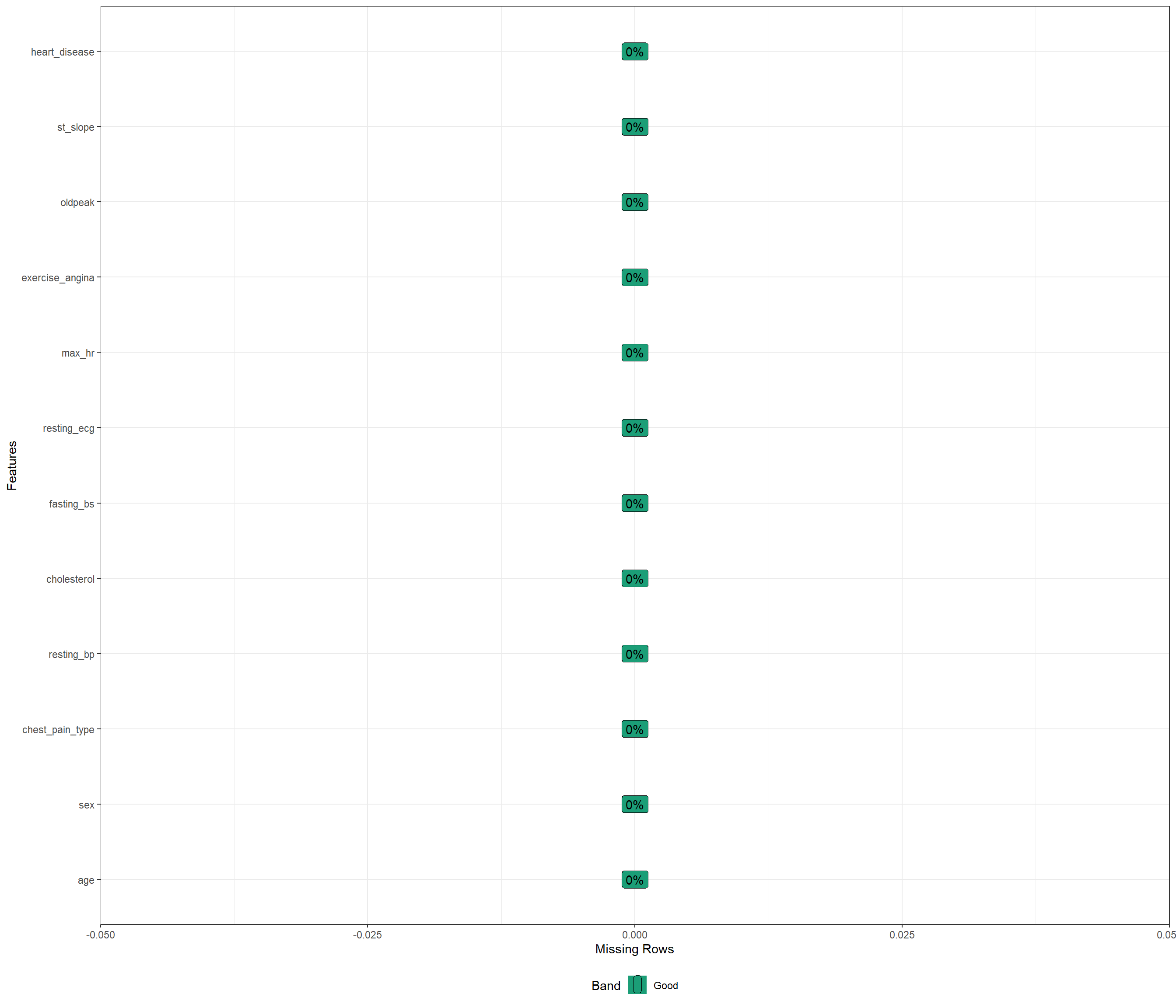
Checking the correlation and distribution of numerical features
heart_train |>
  select(where(is.numeric)) |>
  cor(use = "pairwise.complete.obs") |>
  corrplot::corrplot(method = "number")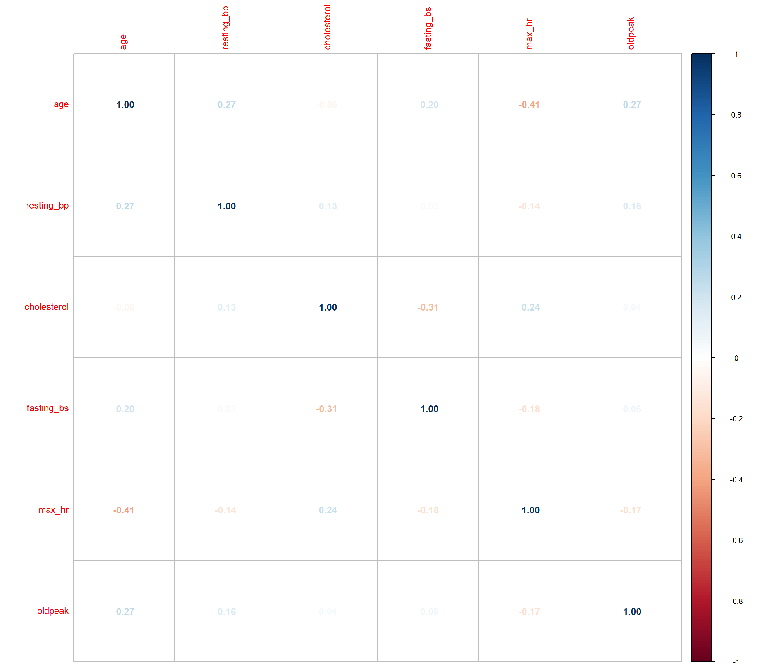
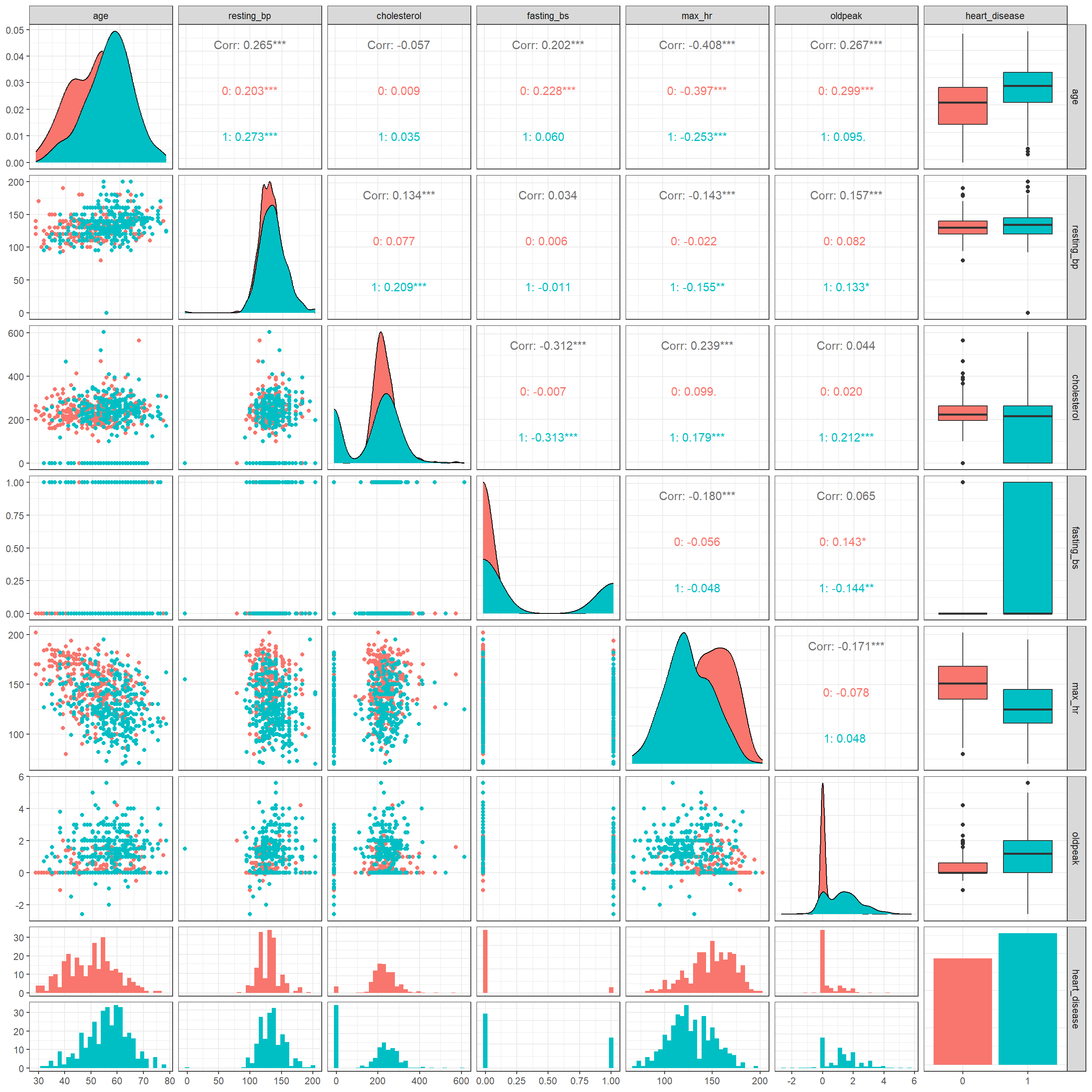
heart_train |>
  select(where(is.numeric), heart_disease) |>
  ggpairs(aes(colour = as_factor(heart_disease))) +
    theme_bw() +
    theme(
      legend.position = "top",
      legend.title = element_blank()
      )
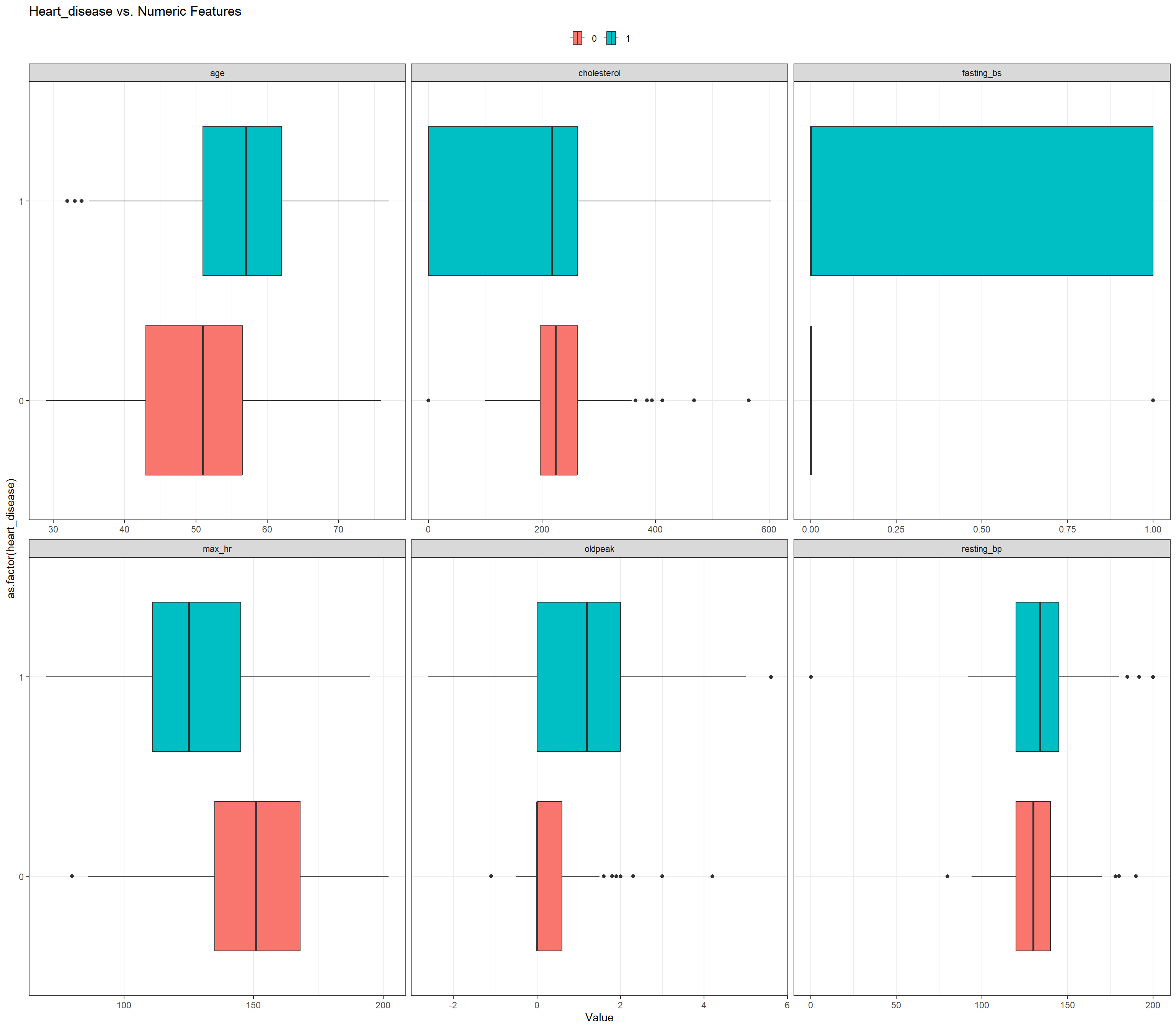
heart_train |>
  select(c(where(is.numeric), heart_disease)) |>
  pivot_longer(-heart_disease,
               names_to = "Feature",
               values_to = "Value") |>
  ggplot(aes(y = as.factor(heart_disease),
             x = Value,
             fill = as.factor(heart_disease))) +
  geom_boxplot() +
  facet_wrap(~Feature,
             scales = "free_x") +
  ggtitle("Heart_disease vs. Numeric Features") +
    theme_bw() +
    theme(
      legend.position = "top",
      legend.title = element_blank()
      )
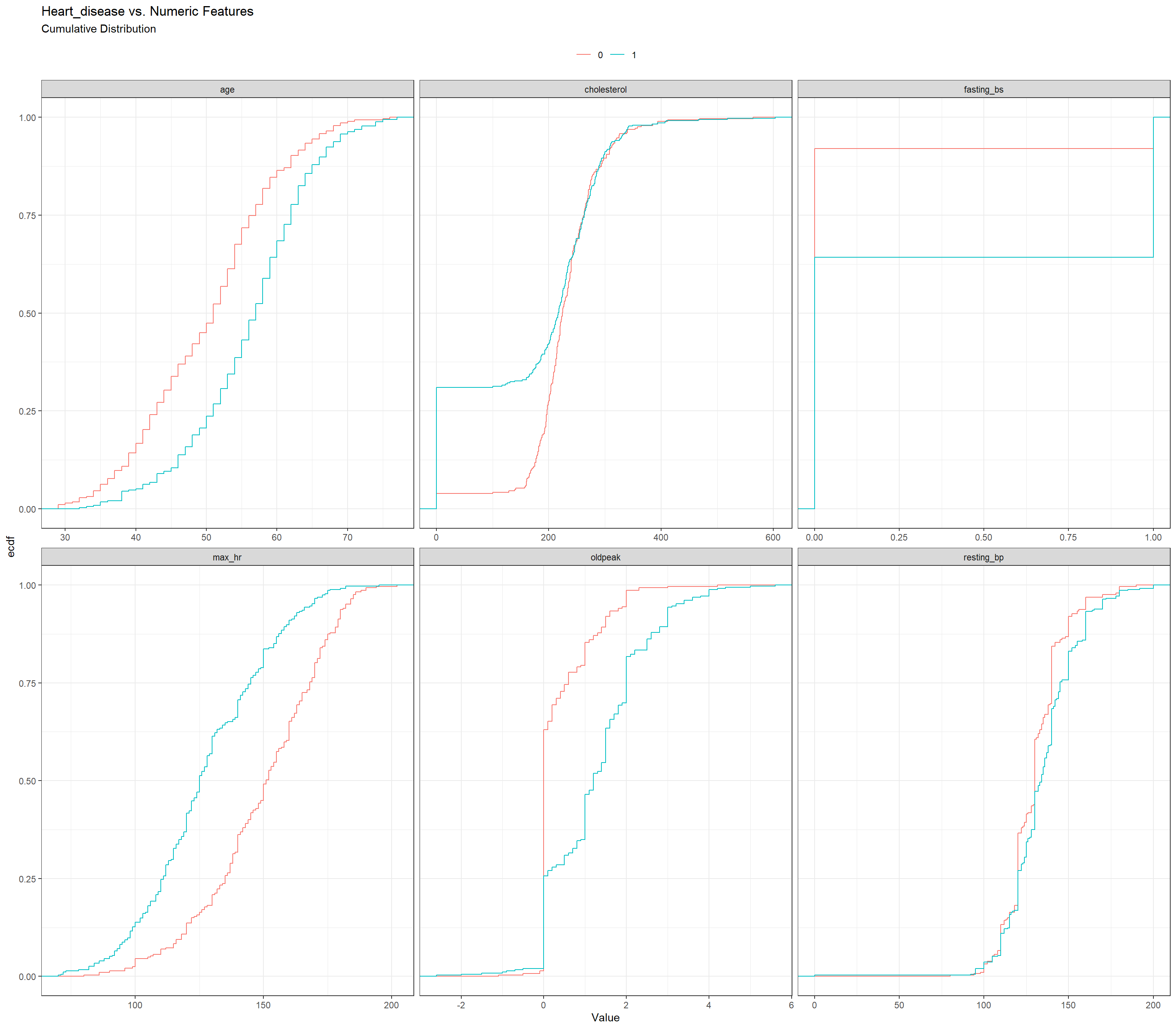
heart_train |>
  select(c(where(is.numeric), heart_disease)) |>
  pivot_longer(-heart_disease,
               names_to = "Feature",
               values_to = "Value") |>
  ggplot(aes(x = Value,
             colour = as.factor(heart_disease))) +
  stat_ecdf() +
  facet_wrap(~Feature, scales = "free_x") +
  labs(title = "Heart_disease vs. Numeric Features",
       subtitle = "Cumulative Distribution") +
    theme_bw() +
    theme(
      legend.position = "top",
      legend.title = element_blank()
      )
grafico_de_barras_das_vars_continuas <-
  function(dados) {
    dados |>
    select(c(where(is.numeric), heart_disease)) |>
    pivot_longer(-heart_disease,
                 names_to = "Feature",
                 values_to = "Value") |>
    dplyr::group_by(Feature) |>
    dplyr::mutate(
      Value = factor(dplyr::ntile(Value, 10),
                     levels = 1:10)
    ) |>
    dplyr::count(heart_disease,
                 Feature,
                 Value) |>
    ggplot(aes(y = (Value),
               x = n,
               fill = as.factor(heart_disease))) +
    geom_col(position = "fill") +
    geom_label(aes(label = n),
               position = position_fill(vjust = 0.5)) +
    facet_wrap(~Feature,
               scales = "free_y",
               ncol = 3) +
    ggtitle("Heart_disease vs. Numeric Features") +
    theme_bw() +
    theme(
      legend.position = "top",
      legend.title = element_blank()
      )
}

grafico_de_barras_das_vars_continuas(heart_train)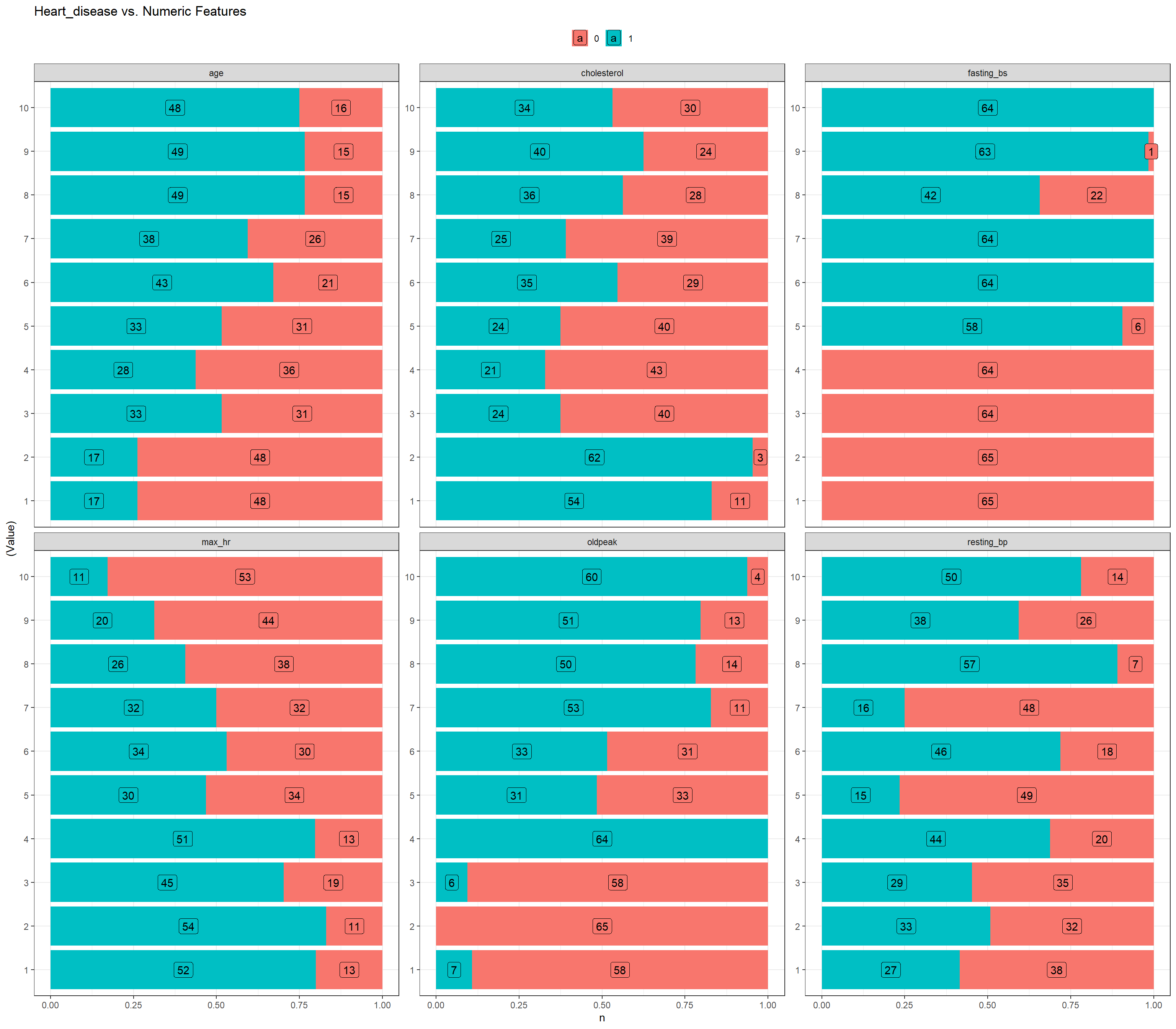
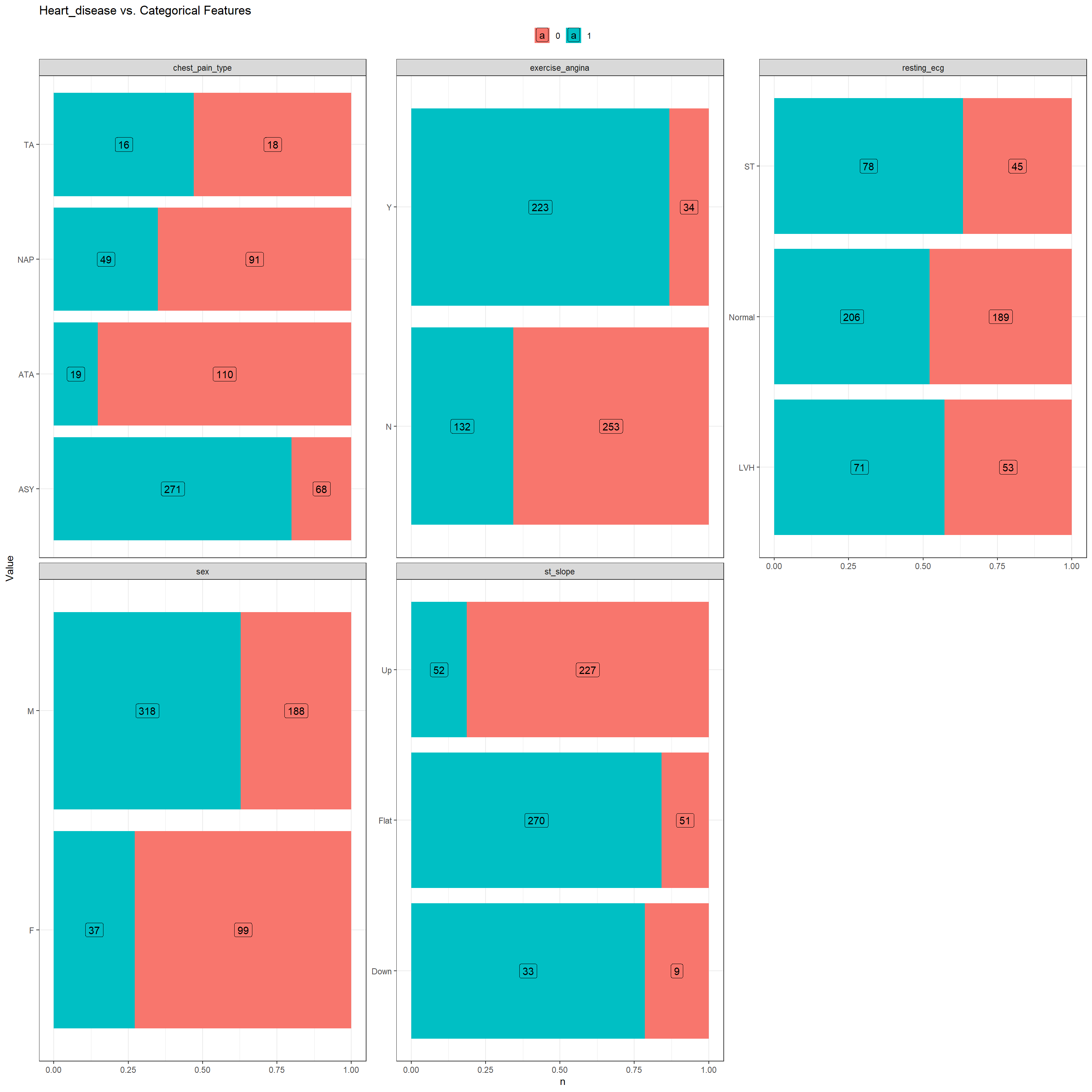
Checking the distribution of categorical features
contagens <-
  heart_train |>
  select(c(where(is.character),
           heart_disease)) |>
  pivot_longer(-heart_disease,
               names_to = "Feature",
               values_to = "Value") |>
  count(heart_disease,
        Feature,
        Value)

# tabela
contagens |>
  pivot_wider(names_from = heart_disease,
              values_from = n) |>
  DT::datatable()
contagens |>
ggplot(aes(y = Value,
x = n,
fill = as.factor(heart_disease))) +
geom_col(position = "fill") +
geom_label(aes(label = n),
position = position_fill(vjust = 0.5)) +
facet_wrap(~Feature,
scales = "free_y",
ncol = 3) +
ggtitle("Heart_disease vs. Categorical Features") +
theme_bw() +
theme(
legend.position = "top",
legend.title = element_blank()
)
Preprocessing and Feature Engineering Steps using Recipes package
For numeric features, the values were normalized, multicollineariry higher than 0.8 were removed and missing values were imputed with median.
For nominal features, missing values were imputed with more frequent value, and all features were transformed in a dummy feature.
Features containing only zero were removed.
The processed dataset can be seen below.
heart_recipe <-
  recipe(formula = heart_disease ~ ., heart_train) |>
  step_normalize(all_numeric_predictors()) |> # normalize all continuous features
  step_corr(all_numeric_predictors(), threshold = .8) |>  # multicollinearity <- r > 0.8
  step_impute_median(all_numeric_predictors()) |>  # Processing missing continuous data - imputing median
  step_impute_mode(all_nominal_predictors()) |> # Processing missing categorical data - imputing more frequent class
  step_zv(all_predictors()) |>  # removing variables that contain only zero (zero variance filter)
  step_dummy(all_nominal_predictors()) # dummy - nominal predictors

# Checking the result of the recipe (and whether the steps worked!)
heart_recipe |>
    prep() |>
    bake(new_data = heart_train) |>
    glimpse()
## Rows: 642
## Columns: 16
## $ age <dbl> -1.4292242, -1.5353499, -0.8985962, 0.0565342, -0.…
## $ resting_bp <dbl> 0.3887070, -0.6642461, -0.1377696, -1.1907226, -0.…
## $ cholesterol <dbl> 0.85757304, 1.32110261, 0.37550228, 0.10665512, 0.…
## $ fasting_bs <dbl> -0.5517274, -0.5517274, -0.5517274, -0.5517274, -0…
## $ max_hr <dbl> 1.339869171, 1.262925121, 1.262925121, 0.185708420…
## $ oldpeak <dbl> -0.8149987, -0.8149987, -0.8149987, -0.8149987, -0…
## $ heart_disease <fct> 0, 0, 0, 0, 0, 0, 0, 0, 0, 0, 0, 0, 0, 0, 0, 0, 0,…
## $ sex_M <dbl> 1, 1, 0, 1, 0, 1, 0, 0, 0, 1, 1, 1, 0, 1, 1, 0, 0,…
## $ chest_pain_type_ATA <dbl> 1, 0, 1, 1, 1, 1, 0, 1, 1, 0, 0, 1, 1, 1, 1, 1, 1,…
## $ chest_pain_type_NAP <dbl> 0, 1, 0, 0, 0, 0, 1, 0, 0, 1, 1, 0, 0, 0, 0, 0, 0,…
## $ chest_pain_type_TA <dbl> 0, 0, 0, 0, 0, 0, 0, 0, 0, 0, 0, 0, 0, 0, 0, 0, 0,…
## $ resting_ecg_Normal <dbl> 1, 1, 1, 1, 1, 1, 0, 1, 1, 1, 1, 1, 1, 1, 1, 0, 1,…
## $ resting_ecg_ST <dbl> 0, 0, 0, 0, 0, 0, 1, 0, 0, 0, 0, 0, 0, 0, 0, 1, 0,…
## $ exercise_angina_Y <dbl> 0, 0, 0, 0, 0, 0, 0, 0, 0, 0, 0, 0, 0, 0, 0, 0, 0,…
## $ st_slope_Flat <dbl> 0, 0, 0, 0, 0, 0, 0, 1, 0, 0, 0, 0, 0, 0, 0, 0, 0,…
## $ st_slope_Up <dbl> 1, 1, 1, 1, 1, 1, 1, 0, 1, 1, 1, 1, 1, 1, 1, 1, 1,…Definition of cross-validation
The cross-validation was set-up in 5 folds.
heart_resamples <-
  vfold_cv(heart_train,
           v = 5,
           strata = heart_disease) # 5 folds

heart_resamples$splits
## [[1]]
## <Analysis/Assess/Total>
## <513/129/642>
##
## [[2]]
## <Analysis/Assess/Total>
## <513/129/642>
##
## [[3]]
## <Analysis/Assess/Total>
## <514/128/642>
##
## [[4]]
## <Analysis/Assess/Total>
## <514/128/642>
##
## [[5]]
## <Analysis/Assess/Total>
## <514/128/642>Modeling - Random Forest
The hyperameters tuned were:
mtry: It refers to an integer for the number of predictors that will be randomly sampled at each split when creating the tree models;
trees: It refers to an integer for the number of trees contained in the ensemble;
min_n: It refers to an integer for the minimum number of data points in a node that are required for the node to be split further.
Model
# Modelo
heart_rf_model <- rand_forest(
  mtry = tune(),
  trees = tune(),
  min_n = tune()
) |>
  set_mode("classification") |>
  set_engine("ranger")
Workflow
# Workflow
heart_rf_wf <- workflow() |>
  add_model(heart_rf_model) |>
  add_recipe(heart_recipe)

heart_rf_wf
## ══ Workflow ════════════════════════════════════════════════════════════════════
## Preprocessor: Recipe
## Model: rand_forest()
##
## ── Preprocessor ────────────────────────────────────────────────────────────────
## 6 Recipe Steps
##
## • step_normalize()
## • step_corr()
## • step_impute_median()
## • step_impute_mode()
## • step_zv()
## • step_dummy()
##
## ── Model ───────────────────────────────────────────────────────────────────────
## Random Forest Model Specification (classification)
##
## Main Arguments:
## mtry = tune()
## trees = tune()
## min_n = tune()
##
## Computational engine: rangerTuning
A Random grid was used for tuning the hyperparameters.
# Tune
heart_grid_rf <- grid_random(
  min_n(range = c(20, 80)),
  mtry(range = c(4, 18)),
  trees(range = c(200, 400))
)

heart_grid_rf |>
  DT::datatable()
doParallel::registerDoParallel(4)
heart_rf_tune_grid <-
tune_grid(
heart_rf_wf,
resamples = heart_resamples,
grid = heart_grid_rf,
metrics = metric_set(roc_auc, accuracy, sensitivity, specificity),
verbose = TRUE
)autoplot(heart_rf_tune_grid) +
theme_bw()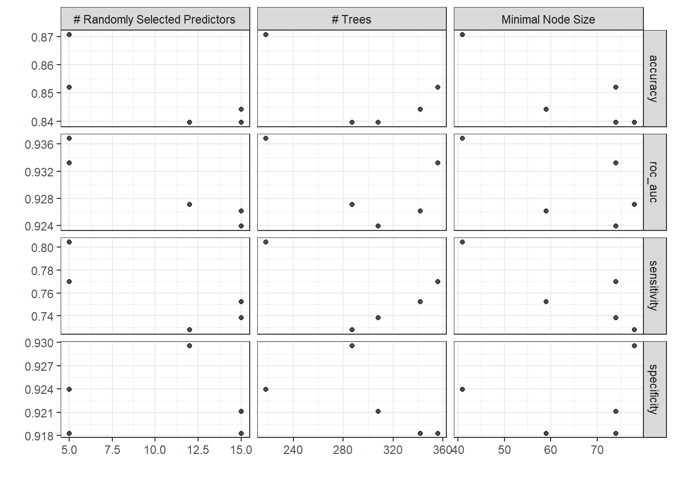
# codes to look metrics --- remove comment to run
# collect_metrics(heart_rf_tune_grid) |>
#   filter(.metric == "roc_auc") |>
#   filter(mean == max(mean))
#
# heart_rf_tune_grid |>
#   select_best(metric = "roc_auc")
#
# show_best(heart_rf_tune_grid, n = 6)
heart_rf_tune_grid |>
select_best(metric = "roc_auc") |>
select(-".config") |>
DT::datatable(caption = htmltools::tags$caption(
style = 'caption-side: top; text-align: left;',
"Best hyperparameters."))Performance
heart_rf_best_params <- select_best(heart_rf_tune_grid,
                                    metric =  "roc_auc")

heart_rf_best_wf <- heart_rf_wf |>
  finalize_workflow(heart_rf_best_params)

heart_rf_last_fit <- last_fit(object = heart_rf_best_wf,
                              split =  heart_initial_split)

heart_test_preds <-
  bind_rows(
    collect_predictions(heart_rf_last_fit) |>
    mutate(modelo = "RandomForest")
)

heart_test_preds |>
  select(
    id, .pred_class, heart_disease
  ) |>
  mutate(
    Prediction = if_else(.pred_class == heart_disease, "RIGHT", "WRONG")
  ) |>
  relocate(Prediction, .before = .pred_class) |>
  DT::datatable()
## ROC
heart_test_preds |>
group_by(modelo) |>
roc_curve(heart_disease, .pred_0) |>
autoplot()+
theme(
legend.position = "top",
legend.title = element_blank()
)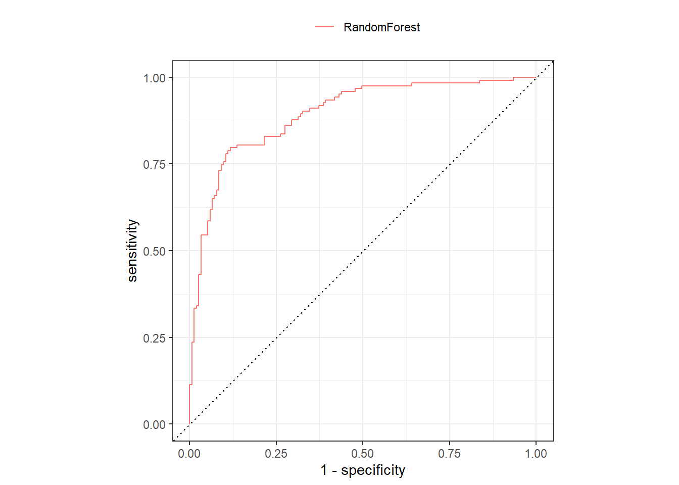
Conclusions
In conclusion, Random Forest proved effective in predicting heart disease. Therefore, this artificial intelligence approach can be implemented in clinical settings to assist healthcare professionals in the early detection of heart disease.
It is noteworthy that the analyses performed herein are not intended to be used in practice. However, these analysis reinforce the utilization of ML algorithm in the health care.
Hope you enjoyed it!😜!
