Using XGboost to Predict Dyspnea in COVID-19 Survivors

By Saulo Gil

January 6, 2024

Introduction

Dyspnea is a medical term that refers to the sensation of shortness of breath or difficulty breathing. It is a common symptom of heart and lung diseases, such as asthma, pneumonia, and chronic obstructive pulmonary disease (COPD).

In the context of COVID-19, dyspnea is one of the most common symptoms experienced by infected individuals, but it remains even after acute COVID-19 is solved. According to a study published in BMC Pulmonary Medicine, 45% of COVID-19 pneumonia survivors admitted to the hospital experience dyspnea even after 1 year from hospital discharge. In this sense, identifying patients at risk of presenting dyspnea is crucial for early management.

XGBoost (eXtreme Gradient Boosting) is a very popular ML algorithm. Its popularity is due to the fact that has recently been dominating applied machine learning and Kaggle competitions for structured or tabular data. Therefore, the implementation of ML algorithm XGBoost in clinical setting may be useful for predicting COVID-19 survivors at the risk of dyspnea following discharge.

Herein, we utilized the XGBoost to predict dyspnea in COVID-19 survivors 6-9 months after hospital discharge

Packages

# Pacotes
library(tidyverse)
library(tidymodels)
library(GGally)
library(DataExplorer)
library(vip)
library(doParallel)

Reading dataset

The dataset consist in a real dataset collected in the largest tertiary hospital of Latin America (Clinical Hospital, School of Medicine of the University of Sao Paulo).

# Lendo a base
dispneia <- read.csv2('df_ajustada.csv')

Spliting dataset - Train/Test

Since our dataset is size-limited, I opted to separate 80% of the sample size for training.

set.seed(32)

dispneia_initial_split <- initial_split(dispneia,
                                        prop = 0.8,
                                        strata = "dispneia")
dispneia_initial_split

## <Training/Testing/Total>
## <592/149/741>

# train and test datasets
dispneia_train <- training(dispneia_initial_split)

dispneia_test <- testing(dispneia_initial_split)

Exploratory analysis

Overview

skimr::skim(dispneia_train)

Table 1: Data summary
Name	dispneia_train
Number of rows	592
Number of columns	47
_______________________
Column type frequency:
character	42
numeric	5
________________________
Group variables	None

Variable type: character

skim_variable	n_missing	complete_rate	min	max	n_unique
idade	0	1.00	5	9	2
sexo	0	1.00	4	6	2
adm_uti	0	1.00	2	3	2
tempo_uti	0	1.00	9	16	3
vmi	0	1.00	2	3	2
tempo_vmi	0	1.00	9	17	3
dispneia	0	1.00	2	3	2
tosse	13	0.98	2	3	2
fraqueza	7	0.99	2	3	2
dific_caminhar	7	0.99	2	3	2
angina	21	0.96	2	3	2
dor_articular	12	0.98	2	3	2
dor_abdominal	12	0.98	2	3	2
diarreia	14	0.98	2	3	2
nausea	9	0.98	2	3	2
perda_consciencia	12	0.98	2	3	2
inapetencia	7	0.99	2	3	2
parestesia	8	0.99	2	3	2
obstrucao_nasal	16	0.97	2	3	2
perda_paladar	25	0.96	2	3	2
anosmia	18	0.97	2	3	2
fadiga	0	1.00	2	3	2
cefaleia	7	0.99	2	3	2
trail_making_a_persistent_fup_incident	73	0.88	2	3	2
perda_memoria	47	0.92	2	3	2
TEPT	11	0.98	2	3	2
perda_auditiva	11	0.98	2	3	2
ruido_ouvido	10	0.98	2	3	2
vertigem	9	0.98	2	3	2
edema	14	0.98	2	3	2
nocturia	15	0.97	2	3	2
dor_corpo	9	0.98	2	3	2
insonia	0	1.00	2	3	2
depressao	64	0.89	2	3	2
ansiedade	64	0.89	2	3	2
tempo_internacao	0	1.00	9	11	2
tabagismo	4	0.99	2	3	2
obesidade	2	1.00	2	3	2
hipertensao	0	1.00	2	3	2
diabetes	0	1.00	2	3	2
gravidade_adm	0	1.00	5	8	4
nivel_atf	3	0.99	5	7	2

Variable type: numeric

skim_variable	n_missing	complete_rate	mean	sd	p0	p25	p50	p75	p100	hist
espiro_cvf_pred	86	0.85	83.46	16.51	22	73.00	84	94.00	132	▁▂▇▆▁
espiro_cvf_vef1_pred	86	0.85	101.78	9.91	43	97.00	103	107.00	129	▁▁▂▇▂
espiro_vef_pred	86	0.85	84.90	17.61	21	75.00	87	96.00	140	▁▂▇▅▁
espiro_pefr_pred	87	0.85	74.68	22.88	9	60.00	76	91.00	133	▁▃▇▆▂
espiro_fef_pred	86	0.85	101.74	39.00	0	75.25	100	125.75	282	▂▇▆▁▁

Missing values

plot_missing(dispneia_train)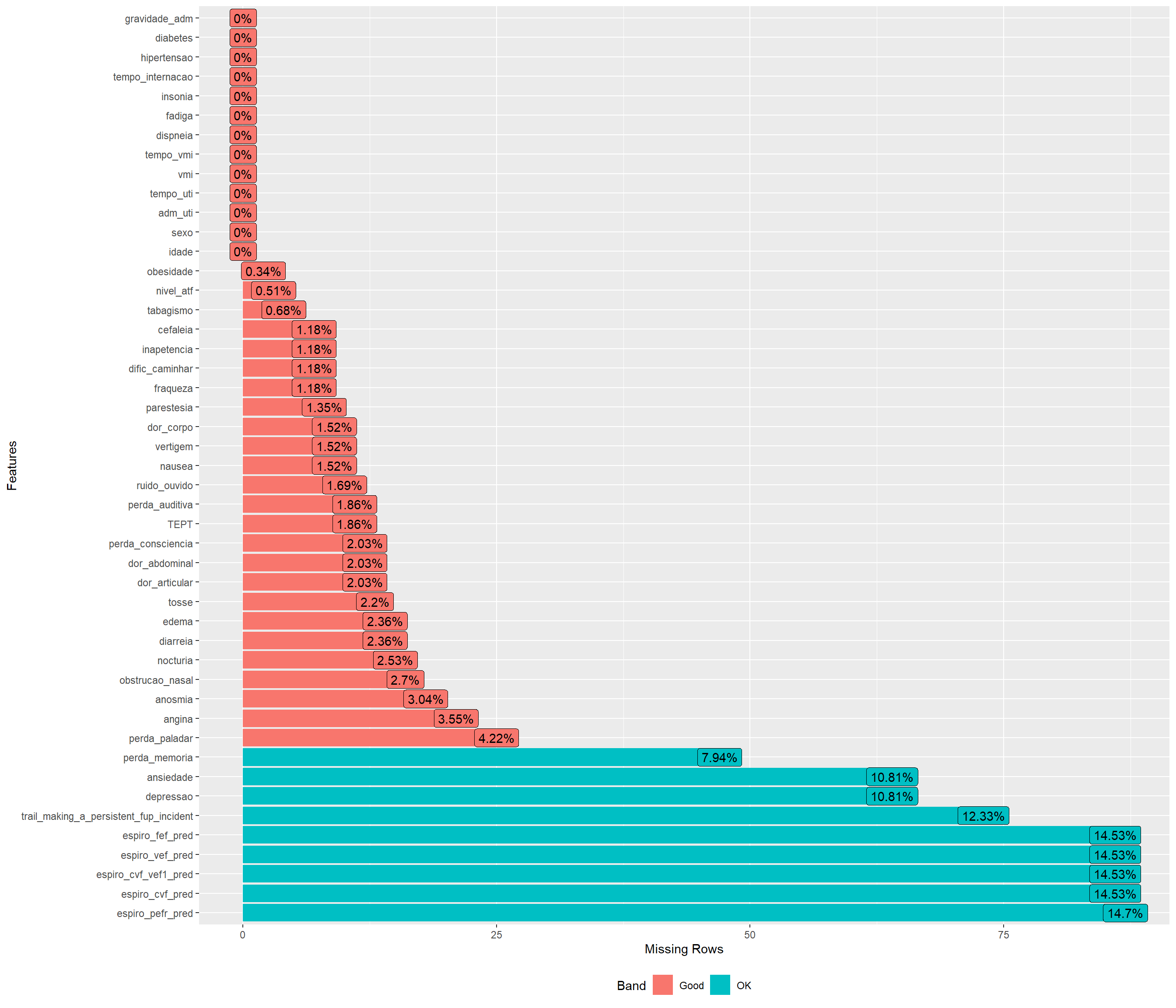

Checking the correlation and distribution of numerical features

dispneia_train |>  
  select(where(is.numeric)) |>  
  cor(use = "pairwise.complete.obs") |> 
  corrplot::corrplot(method = "number")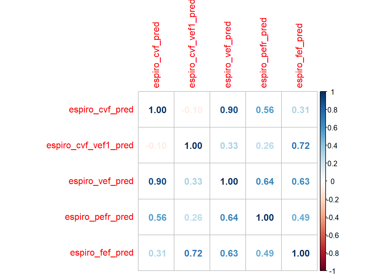

dispneia_train |>  
  select(where(is.numeric), dispneia) |> 
  ggpairs(aes(colour = dispneia))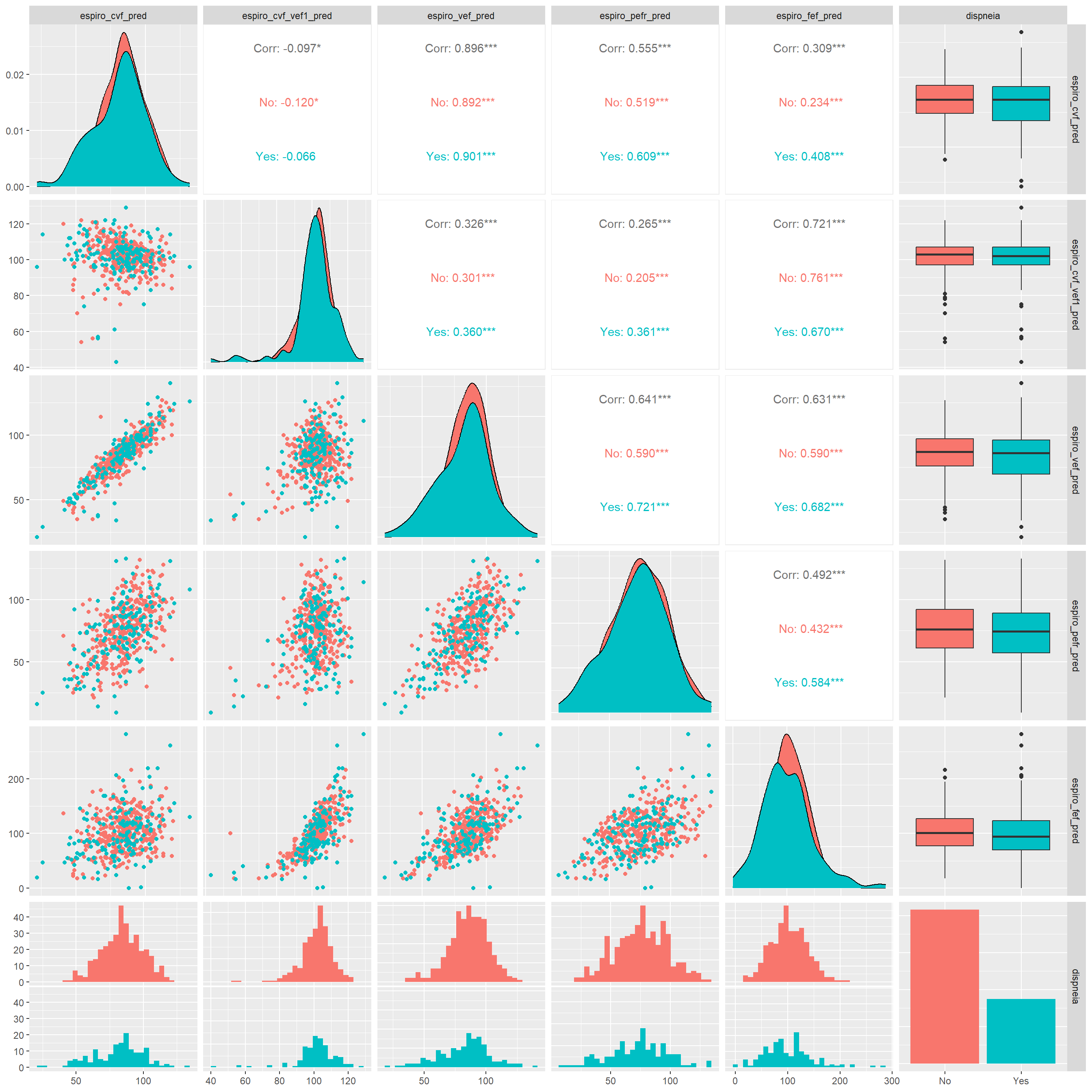

dispneia_train |>  
  select(c(where(is.numeric), dispneia)) |> 
  pivot_longer(-dispneia, 
               names_to = "Feature",
               values_to = "Value") |> 
  ggplot(aes(y = dispneia, 
             x = Value, 
             fill = dispneia)) +
  geom_boxplot() +
  facet_wrap(~Feature,
             scales = "free_x") +
  ggtitle("Dyspnea vs. Numeric Features")

## Warning: Removed 431 rows containing non-finite values (`stat_boxplot()`).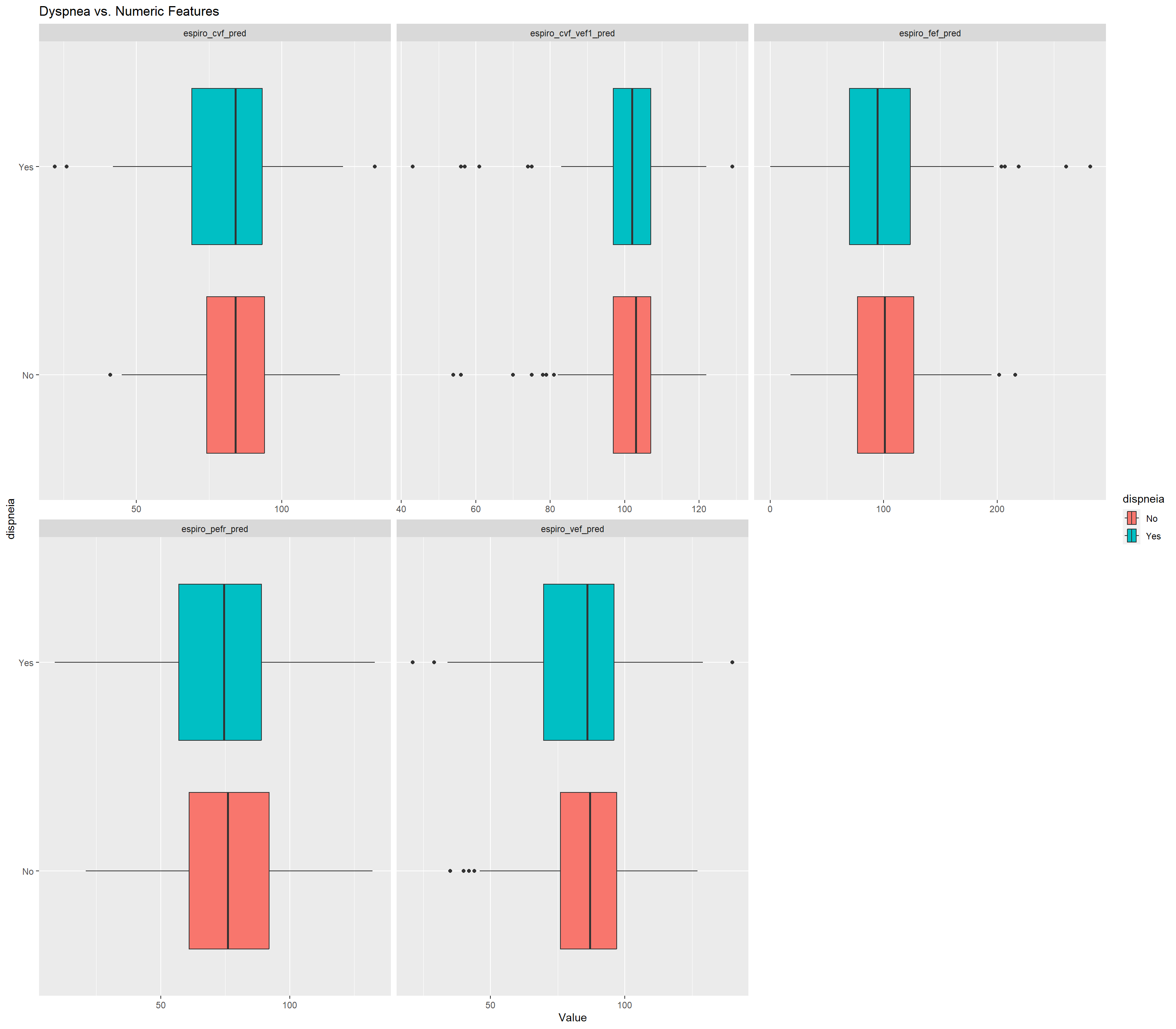

dispneia_train |>  
  select(c(where(is.numeric), dispneia)) |> 
  pivot_longer(-dispneia, 
               names_to = "Feature",
               values_to = "Value") |> 
  ggplot(aes(x = Value, 
             colour = dispneia)) +
  stat_ecdf() +
  facet_wrap(~Feature, scales = "free_x") +
  labs(title = "Dyspnea vs. Numeric Features",
       subtitle = "Cumulative Distribution")

## Warning: Removed 431 rows containing non-finite values (`stat_ecdf()`).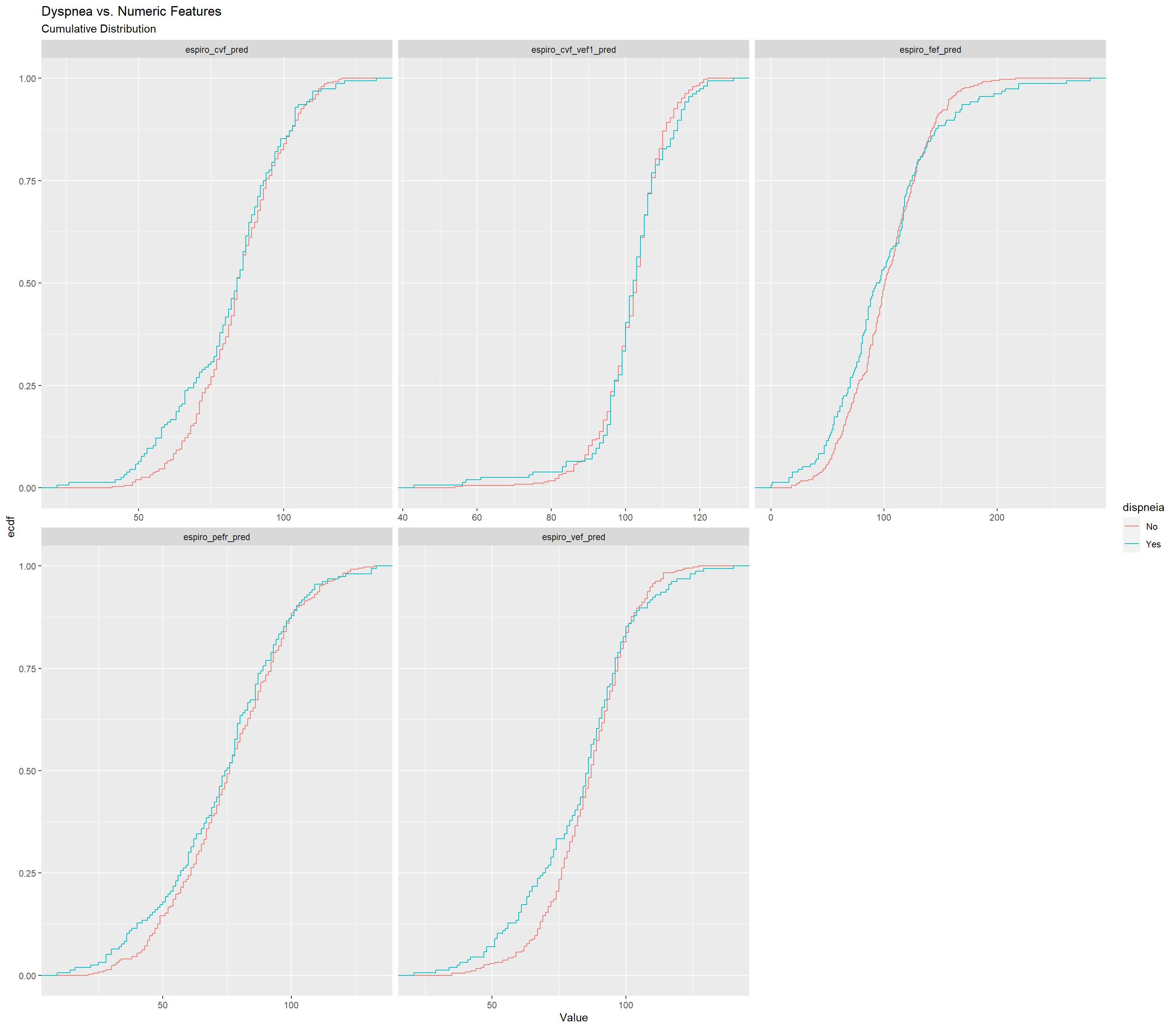

grafico_de_barras_das_vars_continuas <- 
  function(dados) {
    dados |>  
    select(c(where(is.numeric), dispneia)) |> 
    pivot_longer(-dispneia,
                 names_to = "Feature",
                 values_to = "Value") |> 
    dplyr::group_by(Feature) |> 
    dplyr::mutate(
      Value = factor(dplyr::ntile(Value, 10),
                     levels = 1:10)
    ) |> 
    dplyr::count(dispneia, 
                 Feature,
                 Value) |> 
    ggplot(aes(y = (Value),
               x = n,
               fill = dispneia)) +
    geom_col(position = "fill") +
    geom_label(aes(label = n),
               position = position_fill(vjust = 0.5)) +
    facet_wrap(~Feature,
               scales = "free_y",
               ncol = 3) +
    ggtitle("Dyspnea vs. Numeric Features")
}

grafico_de_barras_das_vars_continuas(dispneia_train)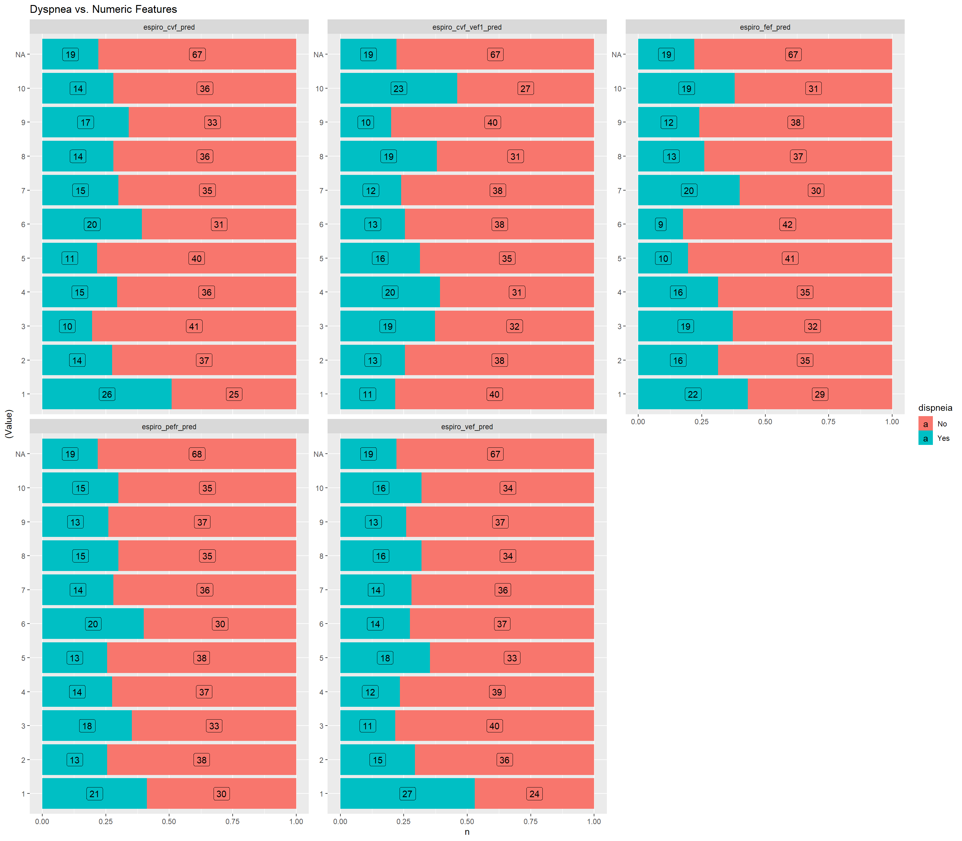

Checking the distribution of categorical features

contagens <- 
  dispneia_train |>  
  select(c(where(is.character),
           dispneia)) |> 
  pivot_longer(-dispneia,
               names_to = "Feature",
               values_to = "Value") |> 
  count(dispneia,
        Feature,
        Value)

# tabela
contagens |> 
  pivot_wider(names_from = dispneia,
              values_from = n) |> 
  DT::datatable()

contagens |> 
  ggplot(aes(y = Value,
             x = n,
             fill = dispneia)) +
  geom_col(position = "fill") +
  geom_label(aes(label = n),
             position = position_fill(vjust = 0.5)) +
  facet_wrap(~Feature,
             scales = "free_y",
             ncol = 3) +
  ggtitle("Dyspnea vs. Categorical Features")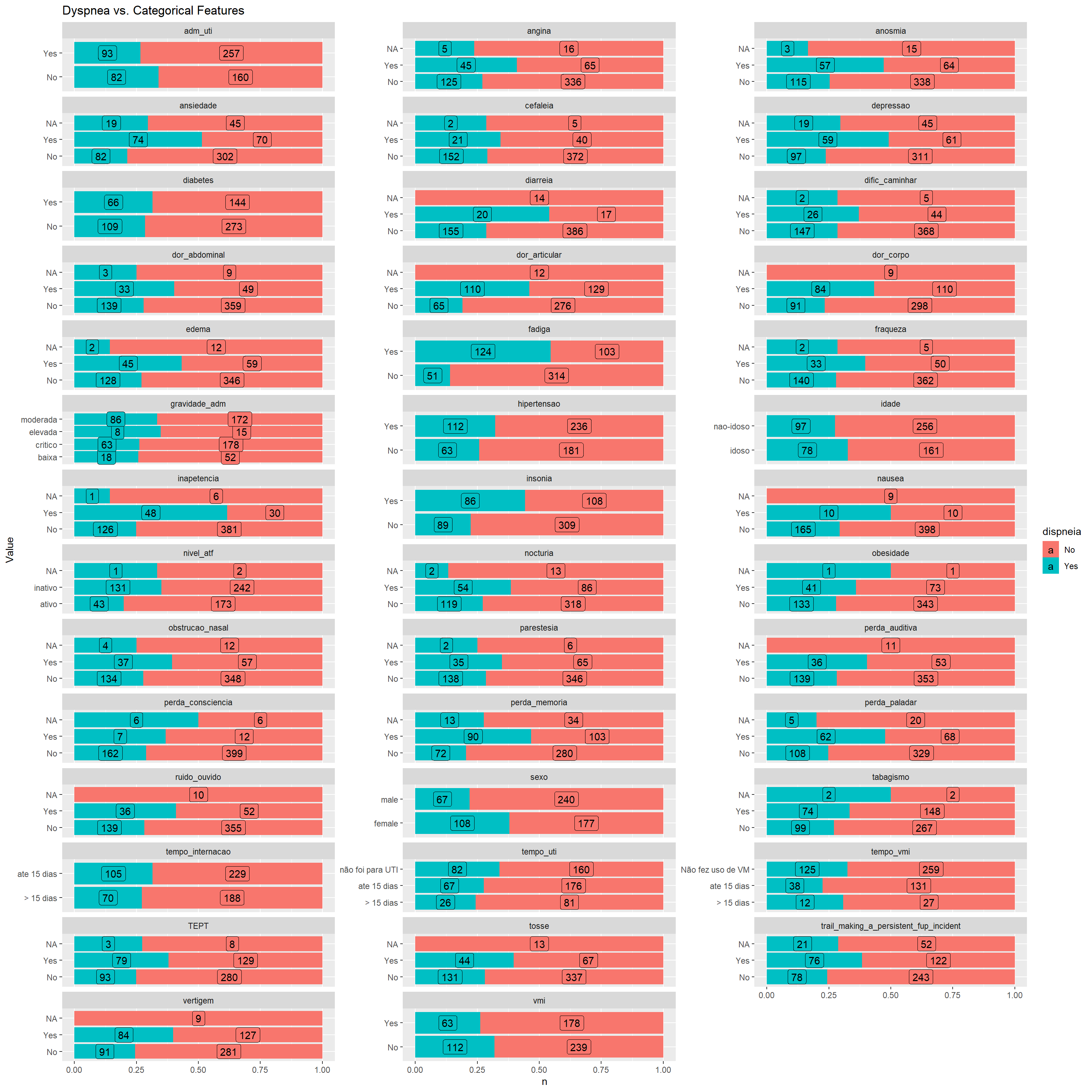

Preprocessing and Feature Engineering Steps using Recipes package

Recipe

For numeric features, the values were normalized, multicollineariry higher than 0.8 were removed and missing values were imputed with median.

For nominal features, missing values were imputed with more frequent value, and all features were transformed in a dummy feature.

Features containing only zero were removed.

The processed dataset can be seen below.

dispneia_recipe <-
  recipe(formula = dispneia ~ ., dispneia_train) |>
  step_normalize(all_numeric_predictors()) |> # normalize all continuous features
  step_corr(all_numeric_predictors(), threshold = .8) |>  # multicollinearity <- r > 0.8
  step_impute_median(all_numeric_predictors()) |>  # Processing missing continuous data - imputing median 
  step_impute_mode(all_nominal_predictors()) |> # Processing missing categorical data - imputing more frequent class
  step_zv(all_predictors()) |>  # removing variables that contain only zero (zero variance filter)
  step_dummy(all_nominal_predictors()) # dummy - nominal predictors

# Checking the result of the recipe (and whether the steps worked!)
dispneia_recipe |> 
    prep() |> 
    bake(new_data = dispneia_train) |> 
    glimpse()

## Rows: 592
## Columns: 50
## $ espiro_cvf_pred                            <dbl> 0.75971560, -0.93614868, -1…
## $ espiro_cvf_vef1_pred                       <dbl> 0.02173529, -0.18006391, 0.…
## $ espiro_pefr_pred                           <dbl> -0.5976043, -2.0833943, 0.2…
## $ espiro_fef_pred                            <dbl> 0.51947489, -1.17275315, -0…
## $ dispneia                                   <fct> No, No, No, No, No, No, No,…
## $ idade_nao.idoso                            <dbl> 1, 0, 1, 0, 1, 0, 1, 0, 0, …
## $ sexo_male                                  <dbl> 1, 0, 1, 1, 1, 1, 0, 1, 0, …
## $ adm_uti_Yes                                <dbl> 1, 1, 1, 1, 1, 1, 1, 1, 1, …
## $ tempo_uti_ate.15.dias                      <dbl> 0, 1, 0, 1, 0, 0, 0, 1, 1, …
## $ tempo_uti_não.foi.para.UTI                 <dbl> 0, 0, 0, 0, 0, 0, 0, 0, 0, …
## $ vmi_Yes                                    <dbl> 1, 1, 1, 1, 1, 1, 1, 1, 0, …
## $ tempo_vmi_ate.15.dias                      <dbl> 0, 1, 0, 1, 0, 1, 1, 0, 0, …
## $ tempo_vmi_Não.fez.uso.de.VM                <dbl> 0, 0, 0, 0, 0, 0, 0, 1, 1, …
## $ tosse_Yes                                  <dbl> 0, 0, 0, 0, 0, 0, 0, 0, 0, …
## $ fraqueza_Yes                               <dbl> 1, 0, 1, 0, 0, 0, 0, 0, 0, …
## $ dific_caminhar_Yes                         <dbl> 0, 0, 1, 0, 0, 0, 0, 0, 0, …
## $ angina_Yes                                 <dbl> 0, 0, 1, 0, 0, 0, 1, 0, 0, …
## $ dor_articular_Yes                          <dbl> 1, 1, 1, 0, 0, 0, 1, 0, 0, …
## $ dor_abdominal_Yes                          <dbl> 0, 0, 0, 1, 0, 0, 0, 0, 0, …
## $ diarreia_Yes                               <dbl> 0, 0, 0, 0, 0, 0, 0, 0, 0, …
## $ nausea_Yes                                 <dbl> 0, 0, 0, 0, 0, 0, 0, 0, 0, …
## $ perda_consciencia_Yes                      <dbl> 0, 1, 0, 0, 0, 0, 0, 0, 0, …
## $ inapetencia_Yes                            <dbl> 0, 0, 0, 0, 0, 0, 0, 0, 0, …
## $ parestesia_Yes                             <dbl> 1, 0, 1, 0, 0, 1, 0, 0, 0, …
## $ obstrucao_nasal_Yes                        <dbl> 0, 0, 0, 0, 0, 0, 0, 1, 0, …
## $ perda_paladar_Yes                          <dbl> 1, 0, 0, 1, 0, 0, 0, 0, 0, …
## $ anosmia_Yes                                <dbl> 0, 0, 0, 0, 0, 0, 0, 0, 0, …
## $ fadiga_Yes                                 <dbl> 0, 1, 0, 1, 1, 0, 1, 0, 0, …
## $ cefaleia_Yes                               <dbl> 0, 0, 0, 0, 0, 0, 0, 0, 0, …
## $ trail_making_a_persistent_fup_incident_Yes <dbl> 1, 0, 0, 0, 0, 0, 1, 0, 0, …
## $ perda_memoria_Yes                          <dbl> 0, 0, 0, 0, 0, 0, 1, 0, 1, …
## $ TEPT_Yes                                   <dbl> 0, 0, 1, 1, 0, 0, 1, 0, 0, …
## $ perda_auditiva_Yes                         <dbl> 0, 0, 0, 0, 0, 0, 0, 0, 0, …
## $ ruido_ouvido_Yes                           <dbl> 0, 0, 1, 0, 0, 0, 1, 0, 0, …
## $ vertigem_Yes                               <dbl> 0, 1, 1, 1, 0, 0, 0, 0, 0, …
## $ edema_Yes                                  <dbl> 1, 0, 0, 0, 0, 1, 1, 0, 0, …
## $ nocturia_Yes                               <dbl> 0, 0, 0, 0, 0, 1, 1, 1, 0, …
## $ dor_corpo_Yes                              <dbl> 0, 0, 0, 0, 1, 1, 1, 1, 1, …
## $ insonia_Yes                                <dbl> 0, 1, 0, 0, 0, 0, 1, 0, 1, …
## $ depressao_Yes                              <dbl> 0, 0, 0, 1, 0, 0, 0, 0, 0, …
## $ ansiedade_Yes                              <dbl> 0, 0, 0, 0, 0, 0, 0, 0, 0, …
## $ tempo_internacao_ate.15.dias               <dbl> 0, 0, 0, 0, 0, 0, 0, 0, 1, …
## $ tabagismo_Yes                              <dbl> 0, 0, 0, 0, 0, 0, 1, 0, 0, …
## $ obesidade_Yes                              <dbl> 0, 0, 0, 0, 0, 0, 0, 0, 0, …
## $ hipertensao_Yes                            <dbl> 1, 1, 0, 1, 1, 1, 1, 0, 1, …
## $ diabetes_Yes                               <dbl> 1, 0, 0, 0, 0, 0, 0, 0, 0, …
## $ gravidade_adm_critico                      <dbl> 1, 1, 1, 1, 1, 1, 1, 1, 0, …
## $ gravidade_adm_elevada                      <dbl> 0, 0, 0, 0, 0, 0, 0, 0, 0, …
## $ gravidade_adm_moderada                     <dbl> 0, 0, 0, 0, 0, 0, 0, 0, 1, …
## $ nivel_atf_inativo                          <dbl> 0, 1, 1, 1, 0, 1, 0, 1, 1, …

Definition of cross-validation

dispneia_resamples <- 
  vfold_cv(dispneia_train,
           v = 5, 
           strata = dispneia) # 5 folds

dispneia_resamples$splits

## [[1]]
## <Analysis/Assess/Total>
## <473/119/592>
## 
## [[2]]
## <Analysis/Assess/Total>
## <473/119/592>
## 
## [[3]]
## <Analysis/Assess/Total>
## <474/118/592>
## 
## [[4]]
## <Analysis/Assess/Total>
## <474/118/592>
## 
## [[5]]
## <Analysis/Assess/Total>
## <474/118/592>

Modeling

XGBoost

The hyperameters tuned were:

boost_tree;
min_n: An integer for the minimum number of data points in a node that is required for the node to be split further;
mtry: A number for the number (or proportion) of predictors that will be randomly sampled at each split when creating the tree models (specific engines only);
trees: An integer for the number of trees contained in the ensemble;
tree_depth: An integer for the maximum depth of the tree (i.e. number of splits) (specific engines only);
learn_rate: A number for the rate at which the boosting algorithm adapts from iteration-to-iteration (specific engines only). This is sometimes referred to as the shrinkage parameter;
loss_reduction: A number for the reduction in the loss function required to split further (specific engines only);
sample_size: A number for the number (or proportion) of data that is exposed to the fitting routine. For xgboost, the sampling is done at each iteration while C5.0 samples once during training.

The tuning process were done in 5 steps.

Step 1 - Number of trees (trees) and learn rate (learn_rate)

Model

# Modelo
dispneia_xgb_model <-
  boost_tree(
  min_n = 15,
  mtry = 0.8,
  trees = tune(),
  tree_depth = 5,
  learn_rate = tune(),
  loss_reduction = 0,
  sample_size = 0.8
) |>
  set_mode("classification") |>
  set_engine("xgboost", count = FALSE)

Workflow

# Workflow
dispneia_xgb_wf <- 
  workflow() |> 
  add_model(dispneia_xgb_model) |> 
  add_recipe(dispneia_recipe)

Tuning

# Tune
dispneia_grid_xgb <-
  expand.grid(
    trees = seq(25, 800, 25),
    learn_rate = seq(0.01, 0.4,0.1)
)

dispneia_grid_xgb |> 
  DT::datatable()

doParallel::registerDoParallel(4)

dispneia_xgb_tune_grid <-
  tune_grid(
  dispneia_xgb_wf,
  resamples = dispneia_resamples,
  grid = dispneia_grid_xgb,
  metrics = metric_set(roc_auc, accuracy, sensitivity, specificity),
  verbose = TRUE
  )

autoplot(dispneia_xgb_tune_grid) +
  theme_bw() +
  theme(legend.position = "top")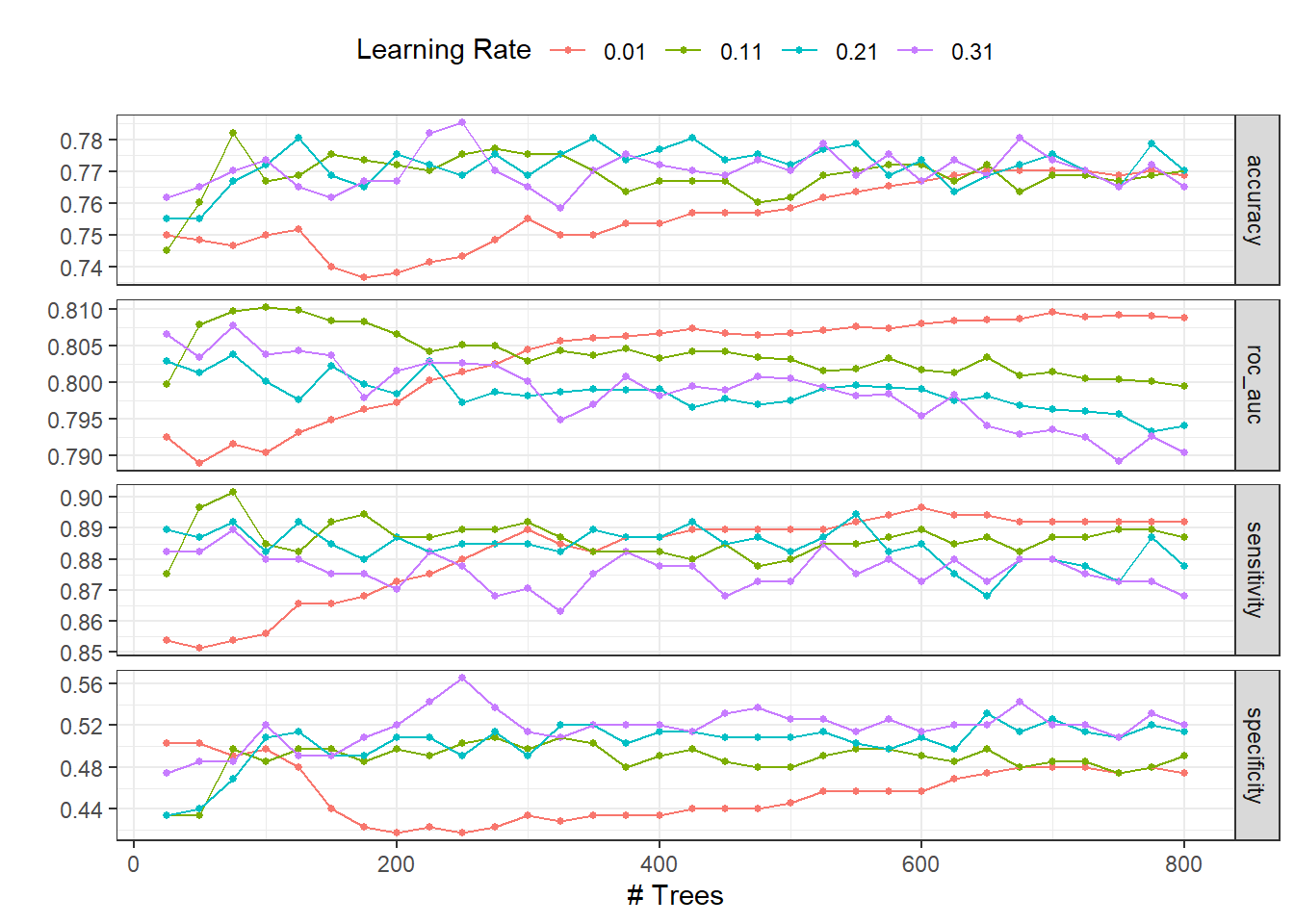

collect_metrics(dispneia_xgb_tune_grid) |> 
  filter(.metric == "roc_auc") |> 
  filter(mean == max(mean))

## # A tibble: 1 × 8
##   trees learn_rate .metric .estimator  mean     n std_err .config               
##   <dbl>      <dbl> <chr>   <chr>      <dbl> <int>   <dbl> <chr>                 
## 1   100       0.11 roc_auc binary     0.810     5  0.0163 Preprocessor1_Model036

dispneia_xgb_tune_grid |> 
  select_best(metric = "roc_auc")

## # A tibble: 1 × 3
##   trees learn_rate .config               
##   <dbl>      <dbl> <chr>                 
## 1   100       0.11 Preprocessor1_Model036

show_best(dispneia_xgb_tune_grid, n = 6)

## # A tibble: 6 × 8
##   trees learn_rate .metric .estimator  mean     n std_err .config               
##   <dbl>      <dbl> <chr>   <chr>      <dbl> <int>   <dbl> <chr>                 
## 1   100       0.11 roc_auc binary     0.810     5  0.0163 Preprocessor1_Model036
## 2   125       0.11 roc_auc binary     0.810     5  0.0161 Preprocessor1_Model037
## 3    75       0.11 roc_auc binary     0.810     5  0.0163 Preprocessor1_Model035
## 4   700       0.01 roc_auc binary     0.810     5  0.0166 Preprocessor1_Model028
## 5   750       0.01 roc_auc binary     0.809     5  0.0162 Preprocessor1_Model030
## 6   775       0.01 roc_auc binary     0.809     5  0.0164 Preprocessor1_Model031

dispneia_best_step1 <-
  dispneia_xgb_tune_grid |>
  select_best(metric = "roc_auc")

# best hiperparameters
glue::glue("The best number of trees was {dispneia_best_step1$trees} and learn_rate was {dispneia_best_step1$learn_rate}.")

## The best number of trees was 100 and learn_rate was 0.11.

Step 2 - Minimal node size (min_n) and depth tree (tree_depth)

Model

# Modelo
dispneia_xgb_model <-
  boost_tree(
  min_n = tune(),
  mtry = 0.8,
  trees = 25,
  tree_depth = tune(),
  learn_rate = 0.31,
  loss_reduction = 0,
  sample_size = 0.8
) |>
  set_mode("classification") |>
  set_engine("xgboost", count = FALSE)

Workflow

# Workflow
dispneia_xgb_wf <- 
  workflow() |> 
  add_model(dispneia_xgb_model) |> 
  add_recipe(dispneia_recipe)

Tuning

# Tune - min_n and tree_depth
dispneia_grid_xgb <-
  expand.grid(
    min_n = seq(1,16,2),
    tree_depth = seq(1,17,4)
)

dispneia_grid_xgb |> 
  DT::datatable()

doParallel::registerDoParallel(4)

dispneia_xgb_tune_grid <-
  tune_grid(
  dispneia_xgb_wf,
  resamples = dispneia_resamples,
  grid = dispneia_grid_xgb,
  metrics = metric_set(roc_auc, accuracy, sensitivity, specificity),
  verbose = TRUE
  )

autoplot(dispneia_xgb_tune_grid) +
  theme_bw() +
  theme(legend.position = "top")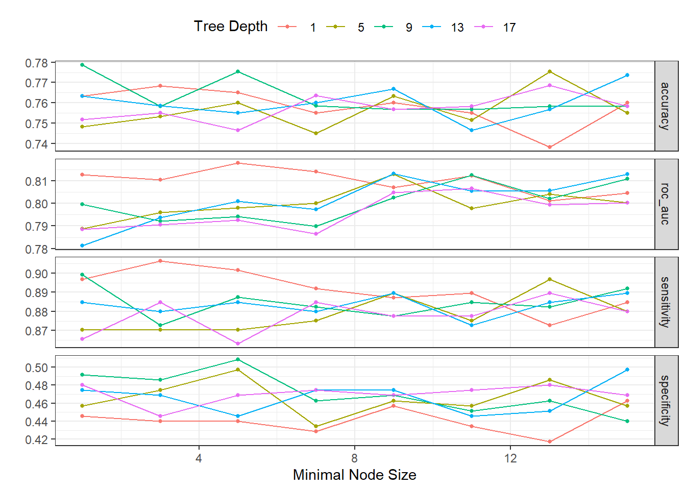

collect_metrics(dispneia_xgb_tune_grid) |> 
  filter(.metric == "roc_auc") |> 
  filter(mean == max(mean))

## # A tibble: 1 × 8
##   min_n tree_depth .metric .estimator  mean     n std_err .config              
##   <dbl>      <dbl> <chr>   <chr>      <dbl> <int>   <dbl> <chr>                
## 1     5          1 roc_auc binary     0.818     5  0.0209 Preprocessor1_Model03

dispneia_xgb_tune_grid |> 
  select_best(metric = "roc_auc")

## # A tibble: 1 × 3
##   min_n tree_depth .config              
##   <dbl>      <dbl> <chr>                
## 1     5          1 Preprocessor1_Model03

show_best(dispneia_xgb_tune_grid, n = 6)

## # A tibble: 6 × 8
##   min_n tree_depth .metric .estimator  mean     n std_err .config              
##   <dbl>      <dbl> <chr>   <chr>      <dbl> <int>   <dbl> <chr>                
## 1     5          1 roc_auc binary     0.818     5  0.0209 Preprocessor1_Model03
## 2     7          1 roc_auc binary     0.814     5  0.0213 Preprocessor1_Model04
## 3     9         13 roc_auc binary     0.813     5  0.0161 Preprocessor1_Model29
## 4     9          5 roc_auc binary     0.813     5  0.0148 Preprocessor1_Model13
## 5    15         13 roc_auc binary     0.813     5  0.0153 Preprocessor1_Model32
## 6     1          1 roc_auc binary     0.813     5  0.0213 Preprocessor1_Model01

dispneia_best_step2 <-
  dispneia_xgb_tune_grid |>
  select_best(metric = "roc_auc")

# best hiperparameters
glue::glue("The best minimal node size was {dispneia_best_step2$min_n} and depth tree was {dispneia_best_step2$tree_depth}.")

## The best minimal node size was 5 and depth tree was 1.

Step 3 - Number for the reduction in the loss function required to split further (loss_reduction)

Model

# Modelo
dispneia_xgb_model <-
  boost_tree(
  min_n = 11,
  mtry = 0.8,
  trees = 25,
  tree_depth = 1,
  learn_rate = 0.31,
  loss_reduction = tune(),
  sample_size = 0.8
) |>
  set_mode("classification") |>
  set_engine("xgboost", count = FALSE)

Workflow

# Workflow
dispneia_xgb_wf <- 
  workflow() |> 
  add_model(dispneia_xgb_model) |> 
  add_recipe(dispneia_recipe)

Tuning

# Tune - min_n and tree_depth
dispneia_grid_xgb <-
  expand.grid(
    loss_reduction = seq(1, 4, 0.04)
)

dispneia_grid_xgb |> 
  DT::datatable()

doParallel::registerDoParallel(4)

dispneia_xgb_tune_grid <-
  tune_grid(
  dispneia_xgb_wf,
  resamples = dispneia_resamples,
  grid = dispneia_grid_xgb,
  metrics = metric_set(roc_auc, accuracy, sensitivity, specificity),
  verbose = TRUE
  )

autoplot(dispneia_xgb_tune_grid) +
  theme_bw()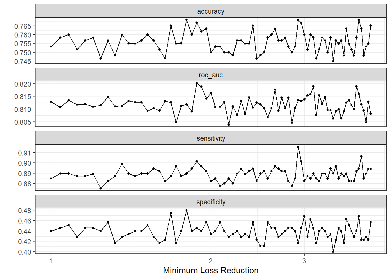

collect_metrics(dispneia_xgb_tune_grid) |> 
  filter(.metric == "roc_auc") |> 
  filter(mean == max(mean))

## # A tibble: 1 × 7
##   loss_reduction .metric .estimator  mean     n std_err .config              
##            <dbl> <chr>   <chr>      <dbl> <int>   <dbl> <chr>                
## 1           1.88 roc_auc binary     0.820     5  0.0195 Preprocessor1_Model23

dispneia_xgb_tune_grid |> 
  select_best(metric = "roc_auc")

## # A tibble: 1 × 2
##   loss_reduction .config              
##            <dbl> <chr>                
## 1           1.88 Preprocessor1_Model23

show_best(dispneia_xgb_tune_grid, n = 6)

## Warning: No value of `metric` was given; metric 'roc_auc' will be used.

## # A tibble: 6 × 7
##   loss_reduction .metric .estimator  mean     n std_err .config              
##            <dbl> <chr>   <chr>      <dbl> <int>   <dbl> <chr>                
## 1           1.88 roc_auc binary     0.820     5  0.0195 Preprocessor1_Model23
## 2           3.76 roc_auc binary     0.819     5  0.0168 Preprocessor1_Model70
## 3           3.12 roc_auc binary     0.819     5  0.0207 Preprocessor1_Model54
## 4           1.92 roc_auc binary     0.819     5  0.0206 Preprocessor1_Model24
## 5           2.64 roc_auc binary     0.818     5  0.0205 Preprocessor1_Model42
## 6           2    roc_auc binary     0.816     5  0.0205 Preprocessor1_Model26

dispneia_best_step3 <-
  dispneia_xgb_tune_grid |>
  select_best(metric = "roc_auc")

# best hiperparameters
glue::glue("The best loss_reduction was {dispneia_best_step3$loss_reduction}.")

## The best loss_reduction was 1.88.

Step 4 - Number (or proportion) of predictors that will be randomly sampled (mtry) and number (or proportion) of data that is exposed to the fitting routine (sample_size)

Model

# Modelo
dispneia_xgb_model <-
  boost_tree(
  min_n = 11,
  mtry = tune(),
  trees = 25,
  tree_depth = 1,
  learn_rate = 0.31,
  loss_reduction = 1.36,
  sample_size = tune()
) |>
  set_mode("classification") |>
  set_engine("xgboost", count = FALSE)

Workflow

# Workflow
dispneia_xgb_wf <- 
  workflow() |> 
  add_model(dispneia_xgb_model) |> 
  add_recipe(dispneia_recipe)

Tuning

# Tune - min_n and tree_depth
dispneia_grid_xgb <-
  expand.grid(
    mtry = seq(0.2, 1.0, 0.2),
    sample_size = seq(0.2, 1.0,by = 0.2)
)

dispneia_grid_xgb |> 
  DT::datatable()

doParallel::registerDoParallel(4)

dispneia_xgb_tune_grid <-
  tune_grid(
  dispneia_xgb_wf,
  resamples = dispneia_resamples,
  grid = dispneia_grid_xgb,
  metrics = metric_set(roc_auc, accuracy, sensitivity, specificity),
  verbose = TRUE
  )

autoplot(dispneia_xgb_tune_grid) +
  theme_bw() +
  theme(legend.position = "top")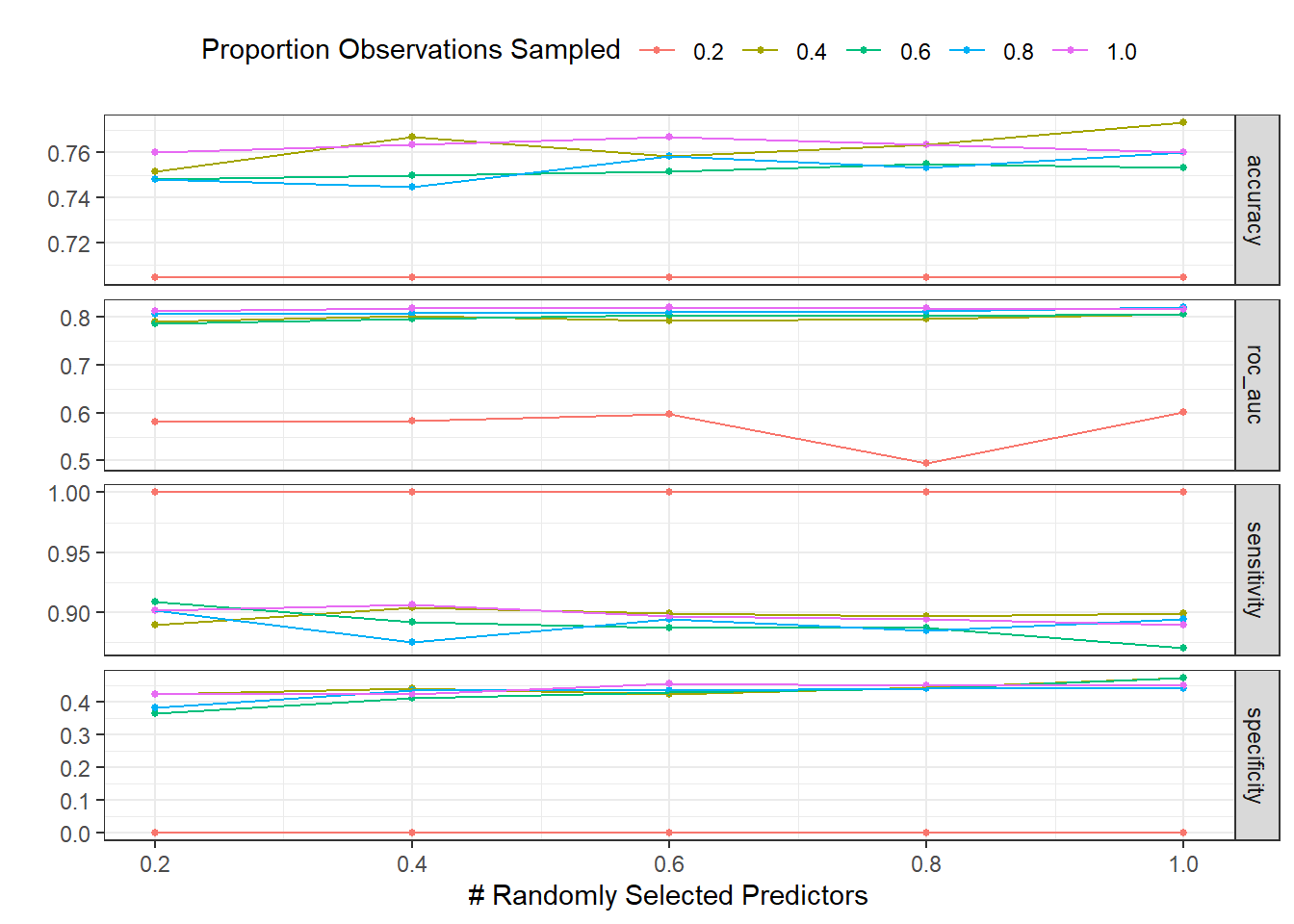

collect_metrics(dispneia_xgb_tune_grid) |> 
  filter(.metric == "roc_auc") |> 
  filter(mean == max(mean))

## # A tibble: 1 × 8
##    mtry sample_size .metric .estimator  mean     n std_err .config              
##   <dbl>       <dbl> <chr>   <chr>      <dbl> <int>   <dbl> <chr>                
## 1   0.6           1 roc_auc binary     0.820     5  0.0217 Preprocessor1_Model23

dispneia_xgb_tune_grid |> 
  select_best(metric = "roc_auc")

## # A tibble: 1 × 3
##    mtry sample_size .config              
##   <dbl>       <dbl> <chr>                
## 1   0.6           1 Preprocessor1_Model23

show_best(dispneia_xgb_tune_grid, n = 6)

## Warning: No value of `metric` was given; metric 'roc_auc' will be used.

## # A tibble: 6 × 8
##    mtry sample_size .metric .estimator  mean     n std_err .config              
##   <dbl>       <dbl> <chr>   <chr>      <dbl> <int>   <dbl> <chr>                
## 1   0.6         1   roc_auc binary     0.820     5  0.0217 Preprocessor1_Model23
## 2   1           0.8 roc_auc binary     0.819     5  0.0197 Preprocessor1_Model20
## 3   0.4         1   roc_auc binary     0.818     5  0.0218 Preprocessor1_Model22
## 4   0.8         1   roc_auc binary     0.818     5  0.0215 Preprocessor1_Model24
## 5   1           1   roc_auc binary     0.817     5  0.0225 Preprocessor1_Model25
## 6   0.2         1   roc_auc binary     0.812     5  0.0227 Preprocessor1_Model21

dispneia_best_step4 <-
  dispneia_xgb_tune_grid |>
  select_best(metric = "roc_auc")

# best hiperparameters
glue::glue("The best number (or proportion) of predictors that will be randomly sampled (mtry) was {dispneia_best_step4$mtry} and the number (or proportion) of data that is exposed to the fitting routine (sample size) was {dispneia_best_step4$sample_size}.")

## The best number (or proportion) of predictors that will be randomly sampled (mtry) was 0.6 and the number (or proportion) of data that is exposed to the fitting routine (sample size) was 1.

Step 5 - Training again learing rate and trees with lower values

Model

# Modelo
dispneia_xgb_model <-
  boost_tree(
  min_n = 11,
  mtry = 0.8,
  trees = tune(),
  tree_depth = 1,
  learn_rate = tune(),
  loss_reduction = 1.36,
  sample_size = 0.8
) |>
  set_mode("classification") |>
  set_engine("xgboost", count = FALSE)

Workflow

# Workflow
dispneia_xgb_wf <- 
  workflow() |> 
  add_model(dispneia_xgb_model) |> 
  add_recipe(dispneia_recipe)

Tuning

# Tune - min_n and tree_depth
dispneia_grid_xgb <-
  expand.grid(
    trees = seq(15, 700, 25),
    learn_rate = seq(0.02, 0.1, 0.02)
)

dispneia_grid_xgb |> 
  DT::datatable()

doParallel::registerDoParallel(4)

dispneia_xgb_tune_grid <-
  tune_grid(
  dispneia_xgb_wf,
  resamples = dispneia_resamples,
  grid = dispneia_grid_xgb,
  metrics = metric_set(roc_auc, accuracy, sensitivity, specificity),
  verbose = TRUE
  )

autoplot(dispneia_xgb_tune_grid) +
  theme_bw() +
  theme(legend.position = "top")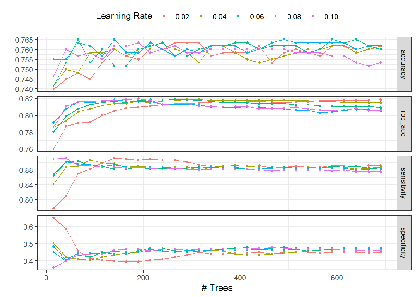

collect_metrics(dispneia_xgb_tune_grid) |> 
  filter(.metric == "roc_auc") |> 
  filter(mean == max(mean))

## # A tibble: 1 × 8
##   trees learn_rate .metric .estimator  mean     n std_err .config               
##   <dbl>      <dbl> <chr>   <chr>      <dbl> <int>   <dbl> <chr>                 
## 1   190        0.1 roc_auc binary     0.820     5  0.0169 Preprocessor1_Model120

dispneia_xgb_tune_grid |> 
  select_best(metric = "roc_auc")

## # A tibble: 1 × 3
##   trees learn_rate .config               
##   <dbl>      <dbl> <chr>                 
## 1   190        0.1 Preprocessor1_Model120

show_best(dispneia_xgb_tune_grid, n = 6)

## Warning: No value of `metric` was given; metric 'roc_auc' will be used.

## # A tibble: 6 × 8
##   trees learn_rate .metric .estimator  mean     n std_err .config               
##   <dbl>      <dbl> <chr>   <chr>      <dbl> <int>   <dbl> <chr>                 
## 1   190       0.1  roc_auc binary     0.820     5  0.0169 Preprocessor1_Model120
## 2   165       0.1  roc_auc binary     0.819     5  0.0175 Preprocessor1_Model119
## 3   290       0.04 roc_auc binary     0.819     5  0.0195 Preprocessor1_Model040
## 4   265       0.06 roc_auc binary     0.819     5  0.0191 Preprocessor1_Model067
## 5   315       0.04 roc_auc binary     0.819     5  0.0196 Preprocessor1_Model041
## 6   290       0.06 roc_auc binary     0.819     5  0.0187 Preprocessor1_Model068

dispneia_best_step5 <-
  dispneia_xgb_tune_grid |>
  select_best(metric = "roc_auc")

# best hiperparameters
glue::glue("Following tunning again, the best number of trees was {dispneia_best_step5$trees} and learn_rate was {dispneia_best_step5$learn_rate}.")

## Following tunning again, the best number of trees was 190 and learn_rate was 0.1.

Final model performance

Model

# Model
dispneia_xgb_final_model <-
  boost_tree(
  min_n = 11,
  mtry = 0.8,
  trees = 565,
  tree_depth = 1,
  learn_rate = 0.02,
  loss_reduction = 1.36,
  sample_size = 0.8
) |>
  set_mode("classification") |>
  set_engine("xgboost", count = FALSE)

Workflow

# Workflow
dispneia_xgb_final_wf <- 
  workflow() |> 
  add_model(dispneia_xgb_final_model) |> 
  add_recipe(dispneia_recipe)

Tuning

# Tune - min_n and tree_depth
dispneia_best_params_xgb <-
  expand.grid(
    min_n = 11,
    mtry = 0.8,
    trees = 565,
    tree_depth = 1,
    learn_rate = 0.02,
    loss_reduction = 1.36,
    sample_size = 0.8
)

dispneia_best_params_xgb |> 
  DT::datatable()

# Desempenho do modelo finaL ----------------------------------------------
dispneia_xgb_final_wf <- 
  dispneia_xgb_final_wf |>
  finalize_workflow(dispneia_best_params_xgb)

dispneia_xgb_last_fit <-
  last_fit(dispneia_xgb_final_wf, dispneia_initial_split)

collect_predictions(dispneia_xgb_last_fit) |> 
  mutate(modelo = "XGBoost") |> 
  group_by(modelo) |> 
  roc_curve(dispneia, .pred_No) |> 
  autoplot() +
  theme_bw() +
  theme(legend.position = "none")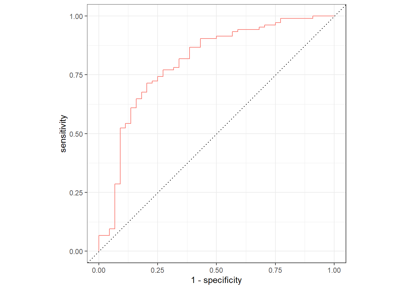

# best hiperparameters
best_roc <- show_best(dispneia_xgb_last_fit)
glue::glue("The best ROC was {round(best_roc$mean,2)}!")

## The best ROC was 0.8!

dispneia_xgb_last_fit_model <- dispneia_xgb_last_fit$.workflow[[1]]$fit$fit

dispneia_xgb_vip <- 
  extract_fit_engine(dispneia_xgb_last_fit)

vip::vip(dispneia_xgb_vip)+
  theme_bw()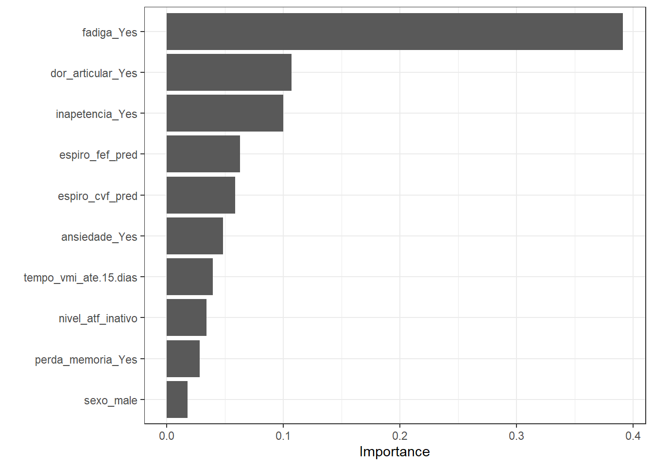

Conclusions

Finally, XGBoost was effective to predict dyspnea in COVID-19 survivors 6-9 months after hospital discharge. Thus, XGBoost implementation in a clinical setting might aid health professionals in the early management of COVID-19 survivors at risk of future dyspnea.

It is noteworthy that the analyses performed herein are not intended to be used in practice. However, these analysis reinforce the utilization of ML algorithm in the health care.

Hope you enjoyed it!😜!

References

Srazzo et al., Long-term dyspnea, regional ventilation distribution and peripheral lung function in COVID-19 survivors: a 1 year follow-up study

An Introduction to Statistical Learning: with Applications in R