Deep Learning - A simple CNN to predict Handwritten Digits
This project consists of implementing a Deep Learning algorithm to detect handwritten digits
By Saulo Gil
July 11, 2024
📒 What is MNIST dataset❓
Introduced by Yann LeCun and colleagues in the 1990s, the MNIST dataset has played a significant role in the development and evaluation of new algorithms in the field of machine learning and deep learning.
The MNIST dataset (Modified National Institute of Standards and Technology dataset) consists of a large database of handwritten digits. Here are some key points about the MNIST dataset:
- Content: It contains 60,000 training images and 10,000 testing images of handwritten digits (0-9). Each image is 28x28 pixels in grayscale.
- Format: The images are standardized, meaning each image is centered and size-normalized. Each pixel value ranges from 0 to 255, where 0 represents white and 255 represents black.
- Usage: The dataset is widely used for benchmarking machine learning algorithms, particularly in the field of image recognition and classification. It’s a common introductory dataset for learning and experimenting with neural networks and other machine learning models.
- Accessibility: The dataset is publicly available and can be easily accessed through various machine learning libraries, such as TensorFlow, PyTorch, and Keras.
📒 What is Convolutional Neural Network - CNN❓
A CNN is a type of deep learning algorithm specifically designed for processing structured grid data, such as images. CNNs are particularly effective for tasks such as image recognition, classification, and detection due to their ability to automatically and adaptively learn spatial hierarchies of features.
Here are some key components and concepts associated with CNNs:
- Convolutional Layers: These layers apply a convolution operation to the input, passing the result to the next layer. Convolutional layers consist of a set of learnable filters (or kernels) that are convolved with the input image to produce feature maps. Each filter detects different features, such as edges, textures, or more complex patterns.
- ReLU Activation Function: After each convolution operation, an activation function like the Rectified Linear Unit (ReLU) is applied. ReLU introduces non-linearity to the model, enabling it to learn more complex patterns.
- Pooling Layers: Also known as subsampling or downsampling, pooling layers reduce the dimensionality of each feature map while retaining the most important information. Max pooling, which takes the maximum value from a set of values in a feature map, is a common type of pooling.
- Fully Connected Layers: These layers are typically used towards the end of the network. Neurons in a fully connected layer have connections to all activations in the previous layer. They are responsible for combining the features extracted by the convolutional and pooling layers to make the final classification or prediction.
- Flattening: Before passing the data to fully connected layers, the output from the convolutional and pooling layers is often flattened into a one-dimensional vector.
- Dropout: This regularization technique involves randomly setting a fraction of input units to zero during training. Dropout helps prevent overfitting by ensuring that the model generalizes better to new data.
- Training: CNNs are trained using backpropagation and gradient descent. The objective is to minimize the loss function by adjusting the weights and biases of the network through iterative updates.
CNNs have achieved state-of-the-art performance in many computer vision tasks, including object detection, facial recognition, and medical image analysis, among others.
Therefore, I utilized a CNN to predict handwritten digits from the MNIST dataset.
Let’s do it❗
👨💻 Programming language
📦 Libraries necessaries
import numpy as np
import keras
from keras import layers
import matplotlib.pyplot as plt
import tensorflow as tf
💻 Preparing the data
# Model / data parameters
num_classes = 10
input_shape = (28, 28, 1)

# Load the data and split it between train and test sets
(x_train, y_train), (x_test, y_test) = keras.datasets.mnist.load_data()

# Scale images to the 0 and 1
x_train = x_train.astype("float32") / 255
x_test = x_test.astype("float32") / 255

# Make sure images have shape (28, 28, 1)
x_train = np.expand_dims(x_train, -1)
x_test = np.expand_dims(x_test, -1)
print("x_train shape:", x_train.shape)
## x_train shape: (60000, 28, 28, 1)print(x_train.shape[0], "train samples")## 60000 train samplesprint(x_test.shape[0], "test samples")## 10000 test samples
# convert class vectors to binary class matrices
y_train = keras.utils.to_categorical(y_train, num_classes)
y_test = keras.utils.to_categorical(y_test, num_classes)
🧐 Looking handwritten digits images
plt.figure()
plt.imshow(x_train[0], cmap=plt.cm.binary)
plt.show()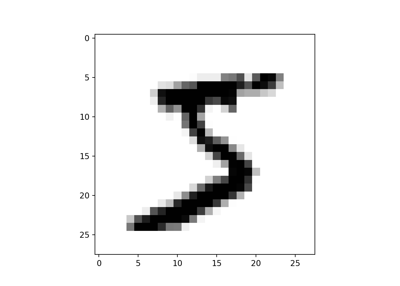
Le’ts see 10 imagens and its labels.
# Ten images and labels
plt.figure(figsize=(15,10))
for i in range(25):
  plt.subplot(5,5,i+1)
  plt.xticks([])
  plt.yticks([])
  plt.imshow(x_train[i], cmap=plt.cm.binary)
  plt.xlabel(f'Label: {np.argmax(y_train[i])}')
plt.show()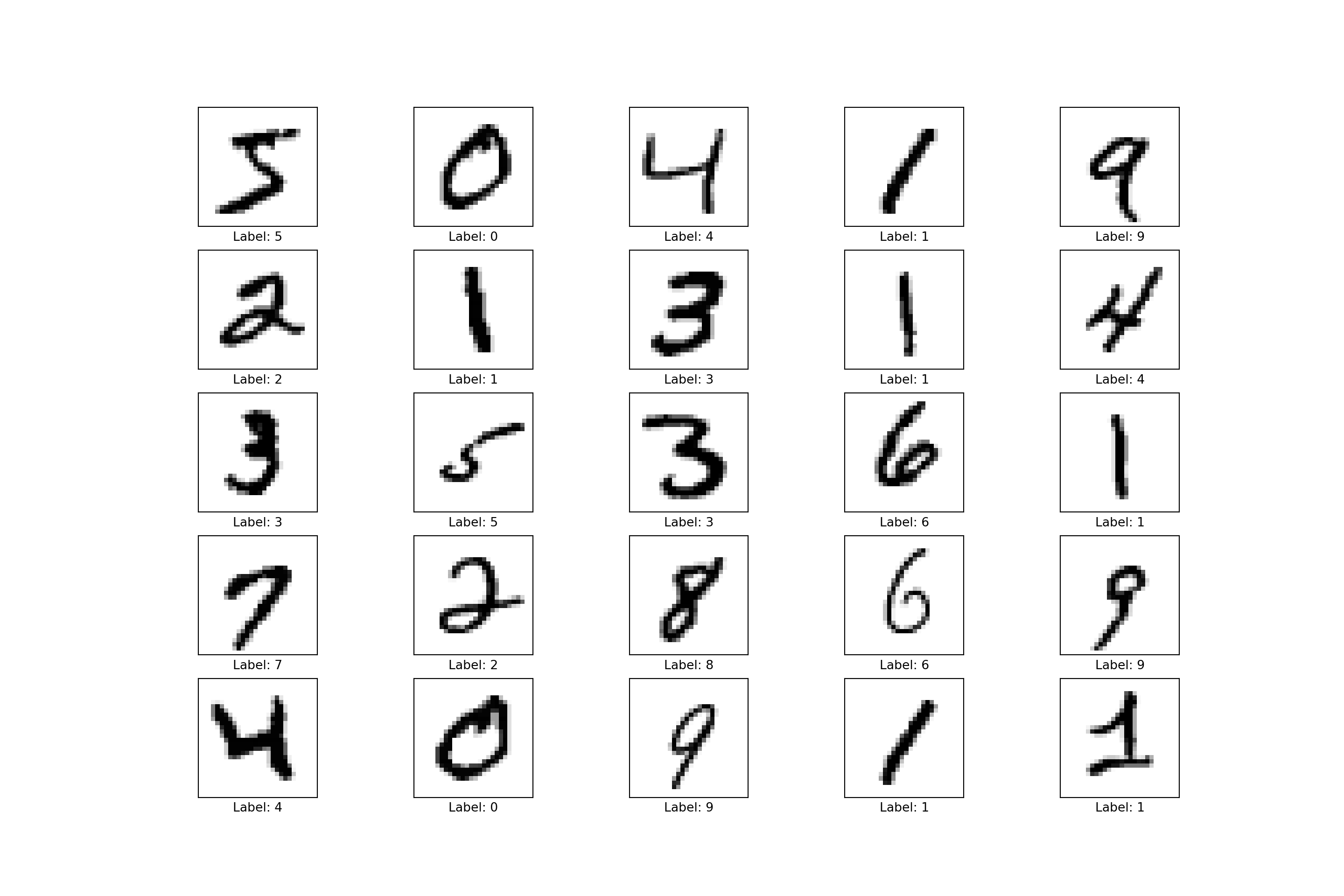
💻🧠 Model - Convolutional Neural Network - CNN
The CNN architecture used was developmented by François Chollet.
This CNN achieved ~99% test accuracy.
The original code is available in the Google Colab.
🤔 Who is François Chollet?
François Chollet is a well-known figure in the field of artificial intelligence and deep learning.
He is the creator of Keras, one of the most popular libraries for deep learning (being used here❗), an interface for the TensorFlow library, among others, that simplifies the process of developing complex neural networks.
He has contributed to various research areas within machine learning and artificial intelligence, including computer vision, natural language processing, and the development of new machine learning architectures.
So, it is a good idea to use a CNN architecture development by him 😜.
Model Summary
┏━━━━━━━━━━━━━━━━━━━━━━━━━━━━━━━━━┳━━━━━━━━━━━━━━━━━━━━━━━━┳━━━━━━━━━━━━━━━┓
┃ Layer (type)                    ┃ Output Shape           ┃       Param # ┃
┡━━━━━━━━━━━━━━━━━━━━━━━━━━━━━━━━━╇━━━━━━━━━━━━━━━━━━━━━━━━╇━━━━━━━━━━━━━━━┩
│ conv2d (Conv2D)                 │ (None, 26, 26, 32)     │           320 │
├─────────────────────────────────┼────────────────────────┼───────────────┤
│ max_pooling2d (MaxPooling2D)    │ (None, 13, 13, 32)     │             0 │
├─────────────────────────────────┼────────────────────────┼───────────────┤
│ conv2d_1 (Conv2D)               │ (None, 11, 11, 64)     │        18,496 │
├─────────────────────────────────┼────────────────────────┼───────────────┤
│ max_pooling2d_1 (MaxPooling2D)  │ (None, 5, 5, 64)       │             0 │
├─────────────────────────────────┼────────────────────────┼───────────────┤
│ flatten (Flatten)               │ (None, 1600)           │             0 │
├─────────────────────────────────┼────────────────────────┼───────────────┤
│ dropout (Dropout)               │ (None, 1600)           │             0 │
├─────────────────────────────────┼────────────────────────┼───────────────┤
│ dense (Dense)                   │ (None, 10)             │        16,010 │
└─────────────────────────────────┴────────────────────────┴───────────────┘
Total params: 34,826 (136.04 KB)
Trainable params: 34,826 (136.04 KB)
Non-trainable params: 0 (0.00 B)
👨💻 Defining a callback, loss function, optimizer and, a model performance metric.
batch_size = 128
epochs = 15

# Callback to interrupt the training when accuracy achieves 99% (implemented just for testing!)
class myCallback(tf.keras.callbacks.Callback):
  def on_epoch_end(self, epoch, logs={}):
    if(logs.get('accuracy')>0.99):
      print("\nReached 99% accuracy so cancelling training!")
      self.model.stop_training = True

callbacks = myCallback()


# Model compile with loss function, optimizer e metrics
model.compile(loss='categorical_crossentropy',
              optimizer='adam',
              metrics=['accuracy'])
🖥️🪫 Training the model
model.fit(x_train, y_train, epochs=epochs, batch_size=batch_size, callbacks=[callbacks], validation_split=0.1, verbose=2)## Epoch 1/15
## 422/422 - 6s - 14ms/step - accuracy: 0.8855 - loss: 0.3728 - val_accuracy: 0.9765 - val_loss: 0.0843
## Epoch 2/15
## 422/422 - 5s - 12ms/step - accuracy: 0.9653 - loss: 0.1134 - val_accuracy: 0.9850 - val_loss: 0.0561
## Epoch 3/15
## 422/422 - 5s - 12ms/step - accuracy: 0.9737 - loss: 0.0843 - val_accuracy: 0.9867 - val_loss: 0.0469
## Epoch 4/15
## 422/422 - 5s - 12ms/step - accuracy: 0.9779 - loss: 0.0700 - val_accuracy: 0.9877 - val_loss: 0.0423
## Epoch 5/15
## 422/422 - 5s - 12ms/step - accuracy: 0.9804 - loss: 0.0624 - val_accuracy: 0.9910 - val_loss: 0.0365
## Epoch 6/15
## 422/422 - 5s - 12ms/step - accuracy: 0.9820 - loss: 0.0579 - val_accuracy: 0.9895 - val_loss: 0.0382
## Epoch 7/15
## 422/422 - 5s - 13ms/step - accuracy: 0.9839 - loss: 0.0508 - val_accuracy: 0.9905 - val_loss: 0.0346
## Epoch 8/15
## 422/422 - 5s - 13ms/step - accuracy: 0.9851 - loss: 0.0477 - val_accuracy: 0.9925 - val_loss: 0.0325
## Epoch 9/15
## 422/422 - 5s - 12ms/step - accuracy: 0.9857 - loss: 0.0454 - val_accuracy: 0.9920 - val_loss: 0.0315
## Epoch 10/15
## 422/422 - 5s - 12ms/step - accuracy: 0.9868 - loss: 0.0412 - val_accuracy: 0.9912 - val_loss: 0.0315
## Epoch 11/15
## 422/422 - 5s - 13ms/step - accuracy: 0.9874 - loss: 0.0398 - val_accuracy: 0.9913 - val_loss: 0.0309
## Epoch 12/15
## 422/422 - 5s - 12ms/step - accuracy: 0.9878 - loss: 0.0378 - val_accuracy: 0.9912 - val_loss: 0.0296
## Epoch 13/15
## 422/422 - 5s - 13ms/step - accuracy: 0.9886 - loss: 0.0348 - val_accuracy: 0.9927 - val_loss: 0.0300
## Epoch 14/15
## 422/422 - 5s - 12ms/step - accuracy: 0.9879 - loss: 0.0360 - val_accuracy: 0.9930 - val_loss: 0.0280
## Epoch 15/15
## 422/422 - 5s - 13ms/step - accuracy: 0.9894 - loss: 0.0326 - val_accuracy: 0.9930 - val_loss: 0.0259
## <keras.src.callbacks.history.History object at 0x0000027131BC2510>🎯 Evaluate the trained model
score = model.evaluate(x_test, y_test, verbose=0)
print("Test loss:", round(score[0], 2))
## Test loss: 0.02print("Test accuracy:", round(score[1], 2))## Test accuracy: 0.99🧐 Looking the predictions
predictions = model.predict(x_test)##
## [1m 1/313[0m [37m━━━━━━━━━━━━━━━━━━━━[0m [1m14s[0m 46ms/step
## [1m 32/313[0m [32m━━[0m[37m━━━━━━━━━━━━━━━━━━[0m [1m0s[0m 2ms/step
## [1m 63/313[0m [32m━━━━[0m[37m━━━━━━━━━━━━━━━━[0m [1m0s[0m 2ms/step
## [1m 90/313[0m [32m━━━━━[0m[37m━━━━━━━━━━━━━━━[0m [1m0s[0m 2ms/step
## [1m127/313[0m [32m━━━━━━━━[0m[37m━━━━━━━━━━━━[0m [1m0s[0m 2ms/step
## [1m165/313[0m [32m━━━━━━━━━━[0m[37m━━━━━━━━━━[0m [1m0s[0m 2ms/step
## [1m205/313[0m [32m━━━━━━━━━━━━━[0m[37m━━━━━━━[0m [1m0s[0m 1ms/step
## [1m244/313[0m [32m━━━━━━━━━━━━━━━[0m[37m━━━━━[0m [1m0s[0m 1ms/step
## [1m283/313[0m [32m━━━━━━━━━━━━━━━━━━[0m[37m━━[0m [1m0s[0m 1ms/step
## [1m313/313[0m [32m━━━━━━━━━━━━━━━━━━━━[0m[37m[0m [1m0s[0m 2ms/step
## [1m313/313[0m [32m━━━━━━━━━━━━━━━━━━━━[0m[37m[0m [1m1s[0m 2ms/stepExample - index 2
np.array(predictions[2])## array([1.3535407e-07, 9.9934298e-01, 4.0317400e-06, 5.9353294e-08,
## 4.7198369e-04, 1.0865199e-06, 2.4188839e-06, 1.4774401e-04,
## 2.8215865e-05, 1.3514803e-06], dtype=float32)np.argmax(predictions[2])## 1As we can see, the highest probability is at index 1 (i.e., 9.99), indicating the value 1.
Let’s see the image❗
plt.figure()
plt.imshow(x_test[2], cmap=plt.cm.binary)
plt.show()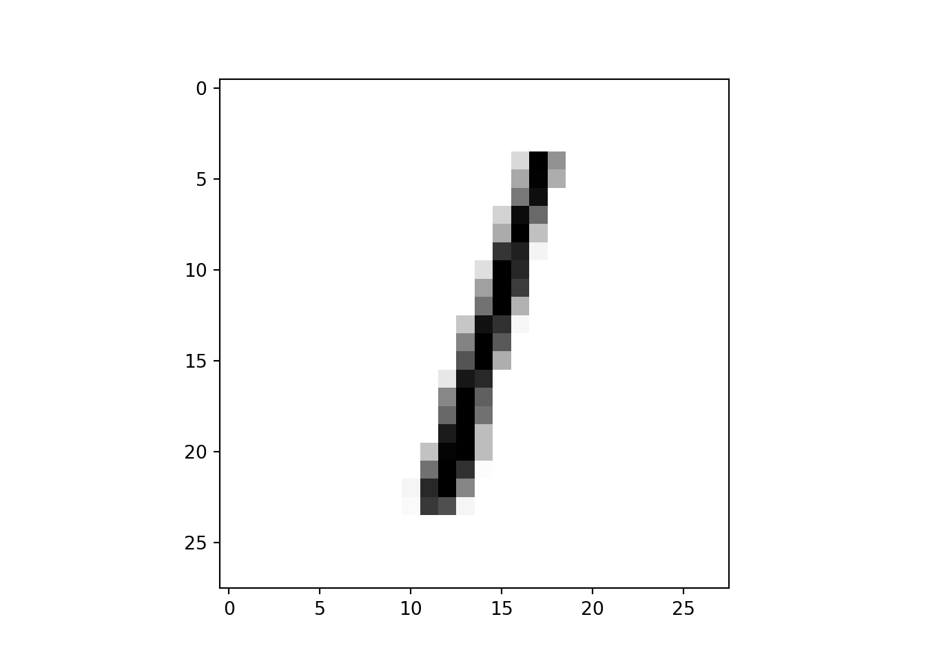
🧐 Now, let’s see 25 examples and predicted labels.
plt.figure(figsize=(15,10))
for i in range(25):
  plt.subplot(5,5,i+1)
  plt.xticks([])
  plt.yticks([])
  plt.imshow(x_test[i], cmap=plt.cm.binary)
  plt.xlabel(f'Predicted label: {np.argmax(predictions[i])}')
plt.show()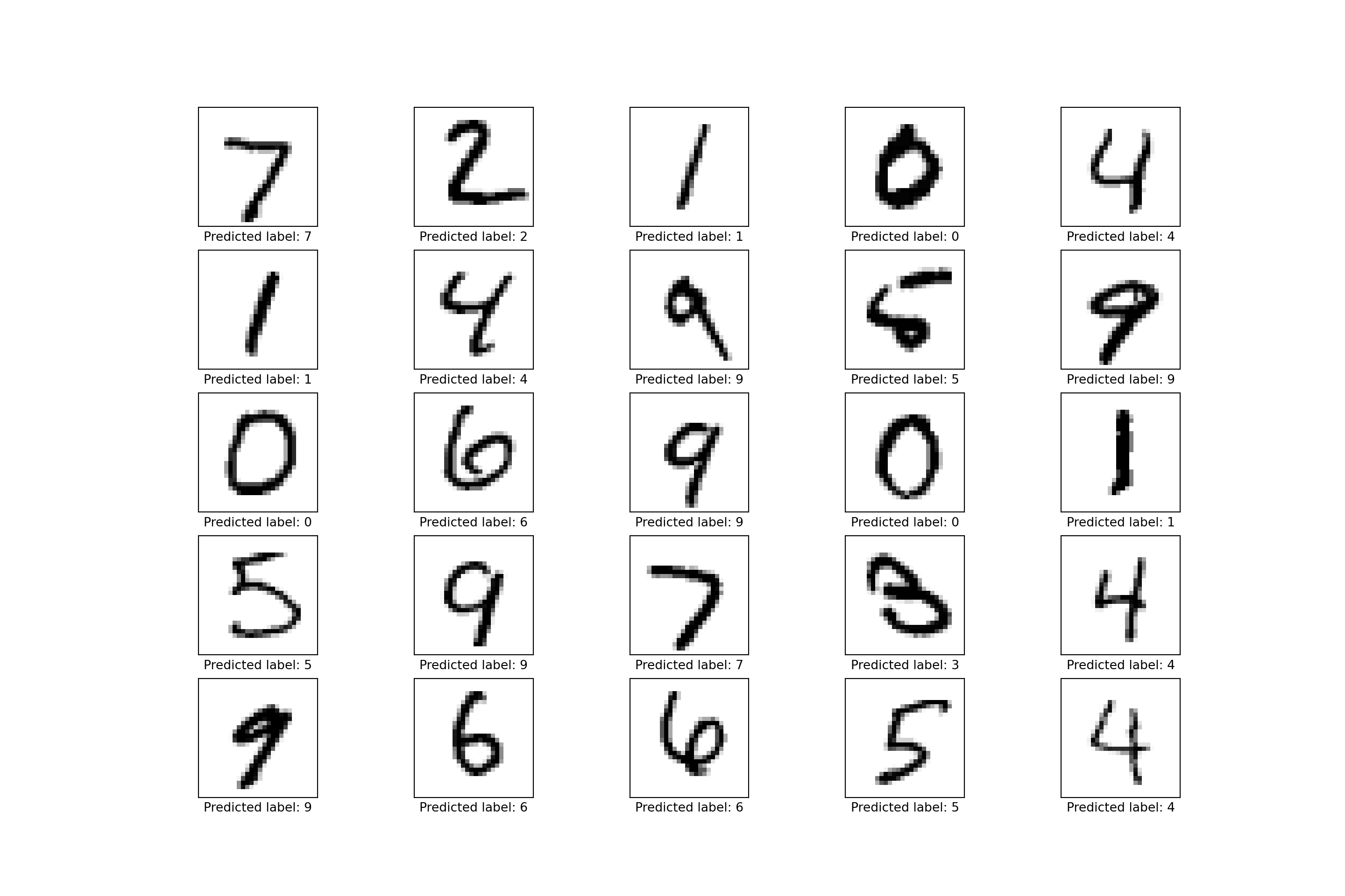
🤓 Conclusion
Indeed, the CNN architecture was able to predict accurately handwritten digits.
This is a simple application of CNNs, but it is noteworthy that this technique has been used to address complex real-world problems.
Hope you enjoyed it!
